A protease family in R
Chymotrypsin cuts a peptide bond with three residues that sit far apart in the
chain and side by side in the folded protein: His57, Asp102 and Ser195. Several
human proteins carry the same domain with one of those three replaced, and cut
nothing. This page starts from fourteen UniProtKB accessions, cuts each chain to
its peptidase S1 domain, aligns the domains, builds a tree, computes two layers
from the alignment, and draws the result with msaviewr, the R htmlwidget.
Every command runs in R, and the last one prints a URL that opens the same view
in a browser.
Prerequisites#
- R 4.3 or newer
- msaviewr:
remotes::install_github("GMOD/JBrowseMSA", subdir = "packages/r-msaview") - Bioconductor:
BiocManager::install(c("Biostrings", "DECIPHER")) - CRAN:
install.packages(c("ape", "jsonlite", "htmlwidgets"))
Every figure below links to the live view it captured.
Where the data comes from#
UniProtKB, twice: once for the feature table that says where each domain starts and which residues carry the charge-relay system, once for the sequences.
- the feature table for all fourteen accessions in one request: https://rest.uniprot.org/uniprotkb/accessions?accessions=P00766,P07477&fields=accession,ft_domain,ft_act_site,ft_disulfid&format=tsv
- the sequences, from the same endpoint: https://rest.uniprot.org/uniprotkb/accessions?accessions=P00766,P07477&format=fasta
- the alignment the commands below write, hosted so the figures can link to it: https://gmod.org/JBrowseMSA/demo/data/proteases/proteases.aln
- its tree: https://gmod.org/JBrowseMSA/demo/data/proteases/proteases.nh
- the layers R computed: https://gmod.org/JBrowseMSA/demo/data/proteases/proteases-layers.json
1. The proteins#
Nine of these fourteen are active peptidases, and five carry the domain with the charge-relay system broken. UniProt records which is which, so the page can check its own answer at the end.
proteins <- data.frame(
  accession = c(
    "P00766", "P07477", "P08246", "P10144", "P07288",
    "P00734", "P00742", "P00747", "P00750",
    "P00738", "P20160", "P22891", "P14210", "P26927"
  ),
  label = c(
    "Chymotrypsinogen", "Trypsin_1", "Elastase", "Granzyme_B", "PSA",
    "Prothrombin", "Factor_X", "Plasminogen", "tPA",
    "Haptoglobin", "Azurocidin", "Protein_Z", "HGF", "MST1"
  )
)
The label becomes the FASTA header, the tree tip and the row the viewer draws down the side. Underscores keep the names through Newick, which reads a space as the end of a name.
The last five are the interesting ones. Haptoglobin binds free hemoglobin, azurocidin kills bacteria by binding their membranes, protein Z carries factor Xa to the phospholipid surface, and HGF and MST1 are growth factors. All five fold like chymotrypsin.
2. One request for the feature table#
UniProt serves any subset of its columns as TSV, so one request covers all fourteen entries and three feature types.
REST <- "https://rest.uniprot.org/uniprotkb/accessions?accessions="
ids <- paste(proteins$accession, collapse = ",")

fields <- "accession,id,protein_name,ft_domain,ft_act_site,ft_disulfid"
features <- read.delim(
  url(paste0(REST, ids, "&fields=", fields, "&format=tsv")),
  quote = "", check.names = FALSE
)
features <- features[match(proteins$accession, features$Entry), ]
Each feature column holds one long string, so two small parsers turn it into numbers:
# "DOMAIN 364..618; /note="Peptidase S1"" -> c(364, 618)
s1_domain <- function(text) {
  m <- regmatches(text, regexpr('DOMAIN (\\d+)\\.\\.(\\d+); /note="Peptidase S1"', text))
  as.integer(regmatches(m, gregexpr("\\d+", m))[[1]])
}
# "ACT_SITE 406; ... ACT_SITE 462; ..." -> c(406, 462, 568)
positions <- function(text, key) {
  m <- regmatches(text, gregexpr(paste0(key, " (\\d+)"), text))[[1]]
  as.integer(sub(paste0(key, " "), "", m))
}

domains <- lapply(features[["Domain [FT]"]], s1_domain)
proteins$start <- vapply(domains, `[`, integer(1), 1)
proteins$end <- vapply(domains, `[`, integer(1), 2)
proteins$act <- lapply(features[["Active site"]], positions, "ACT_SITE")
protein domain residues active_site
Chymotrypsinogen 16..243 228 57, 102, 195
Trypsin_1 24..244 221 63, 107, 200
Elastase 30..247 218 70, 117, 202
Granzyme_B 21..245 225 64, 108, 203
PSA 25..258 234 65, 120, 213
Prothrombin 364..618 255 406, 462, 568
Factor_X 235..467 233 276, 322, 419
Plasminogen 581..808 228 622, 665, 760
tPA 311..561 251 357, 406, 513
Haptoglobin 162..404 243 none
Azurocidin 27..244 218 none
Protein_Z 175..400 226 none
HGF 495..721 227 none
MST1 484..709 226 noneThe domain starts at residue 16 of chymotrypsinogen and at residue 581 of plasminogen, so residue 195 means a different thing in each row. The five rows with no active site are the five proteins named above.
3. Cut each chain to its domain#
subseq takes the start and end vectors whole, one call for all fourteen.
fasta <- "proteases-full.fasta"
download.file(paste0(REST, ids, "&format=fasta"), fasta, quiet = TRUE)
full <- readAAStringSet(fasta)
names(full) <- sub("^[a-z]+\\|([A-Z0-9]+)\\|.*$", "\\1", names(full))
full <- full[proteins$accession]

s1 <- subseq(full, start = proteins$start, end = proteins$end)
names(s1) <- proteins$label
full chains 245-810 aa, S1 domains 218-255 aaThe chains differ by a factor of three, because prothrombin and plasminogen carry Gla and kringle domains ahead of the peptidase. The domains differ by 37 residues.
4. Align the domains#
aln <- AlignSeqs(s1, verbose = FALSE)
writeXStringSet(aln, "proteases.aln")
alignment: 14 rows x 297 columns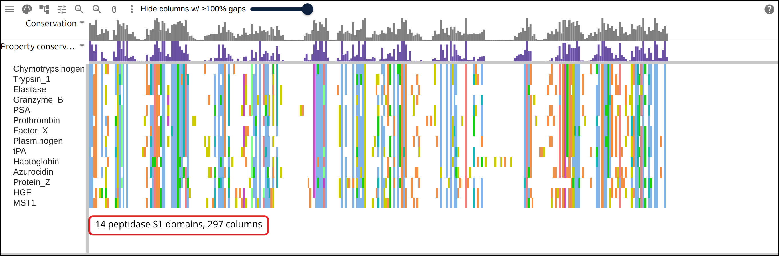
AlignSeqs, in the order the accession table lists
them: the nine active peptidases first, the five without a charge-relay system
last. The gaps are the loops, which differ in length between families.5. A tree from the alignment#
DistanceMatrix reads the alignment, nj builds the tree, and ladderize
sorts each node so the smaller clade comes first.
tree <- ladderize(nj(as.dist(DistanceMatrix(aln, verbose = FALSE))))
write.tree(tree, "proteases.nh")
An ape::phylo goes into msaview() as it is, along with the AAStringSet:
msaview(msa = aln, tree = tree, color_scheme = "clustalx_protein_dynamic")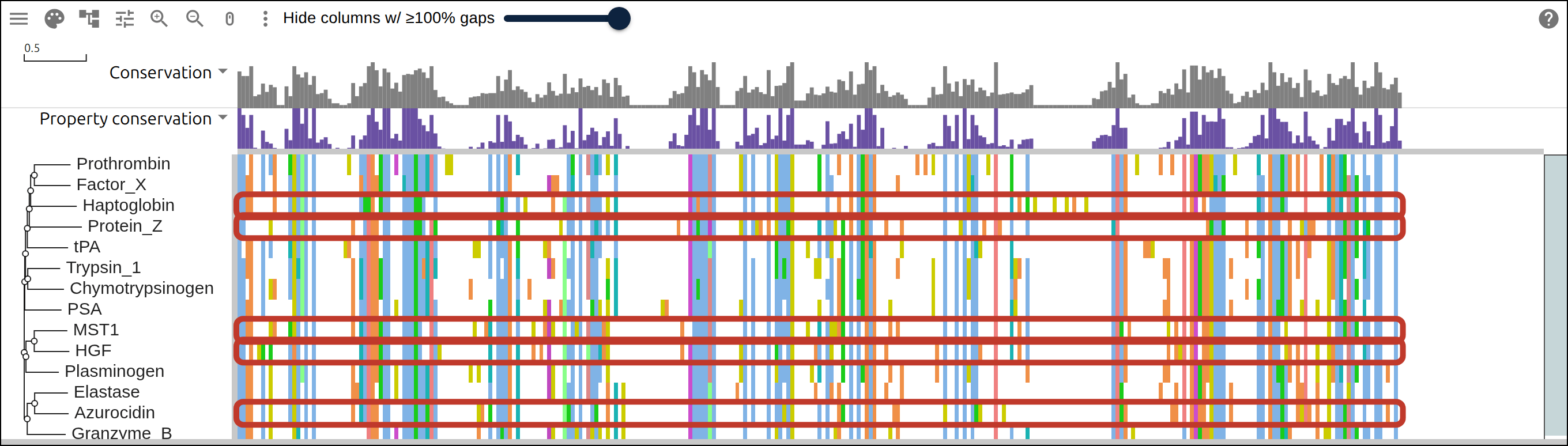
6. A track from R’s own numbers#
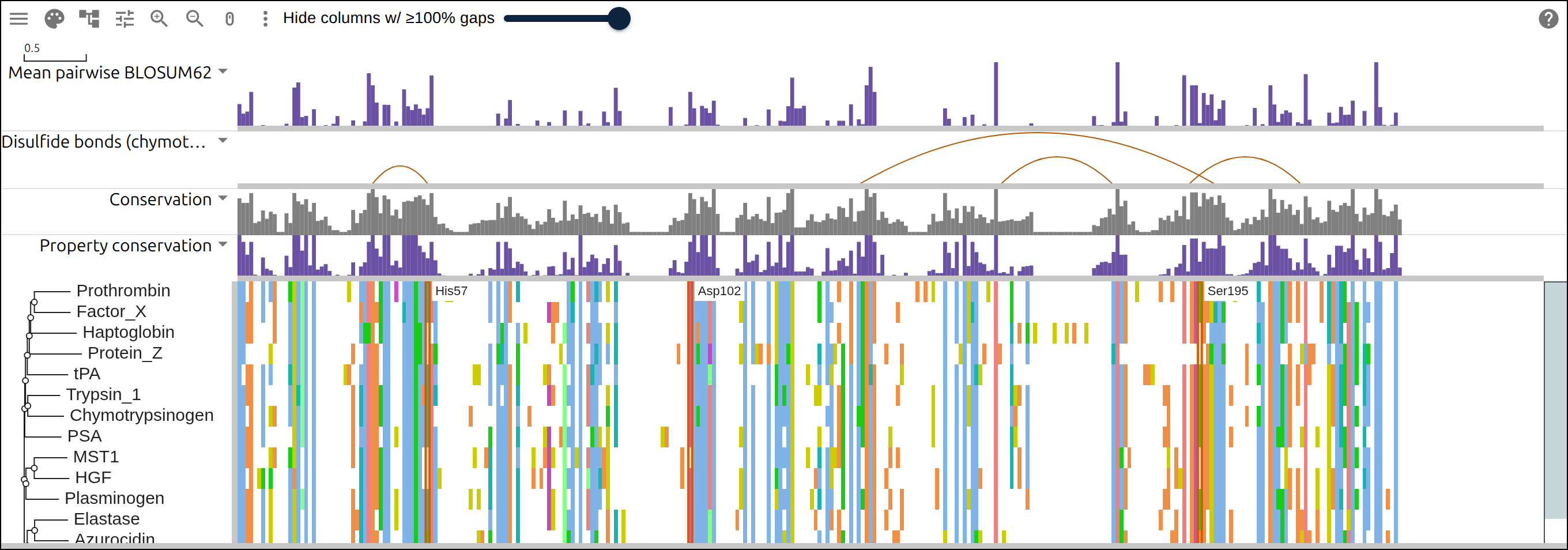
The viewer computes a conservation track from the alignment, which counts how often a column agrees. A substitution matrix answers a different question: it scores a conserved cysteine at 9 and a conserved alanine at 4, because a cysteine that survives everywhere is rarer than an alanine that does.
data(BLOSUM62, package = "Biostrings")
m <- as.matrix(aln)
pairs <- combn(nrow(m), 2)
blosum <- apply(m, 2, function(column) {
  a <- column[pairs[1, ]]
  b <- column[pairs[2, ]]
  keep <- a %in% rownames(BLOSUM62) & b %in% rownames(BLOSUM62)
  if (!any(keep)) 0 else mean(BLOSUM62[cbind(a[keep], b[keep])])
})
column_tracks takes the vector as one bar per column, scaled by max:
blosum_track <- list(
  id = "blosum", name = "Mean pairwise BLOSUM62", kind = "bar",
  values = pmax(blosum, 0), max = 9, color = "#6a51a3", height = 60
)
7. The disulfide bonds, as arcs#
The feature table already holds them. Chymotrypsinogen has five, and four lie inside the domain the alignment covers.
disulfides <- function(text) {
  m <- regmatches(text, gregexpr("DISULFID (\\d+)\\.\\.(\\d+)", text))[[1]]
  matrix(as.integer(unlist(regmatches(m, gregexpr("\\d+", m)))), ncol = 2, byrow = TRUE)
}

ref <- which(proteins$label == "Chymotrypsinogen")
ss <- disulfides(features[["Disulfide bond"]][ref])
ss <- ss[ss[, 1] >= proteins$start[ref] & ss[, 2] <= proteins$end[ref], , drop = FALSE]
bonds <- data.frame(
  start = ss[, 1] - proteins$start[ref] + 1,
  end = ss[, 2] - proteins$start[ref] + 1
)

ss_track <- list(
  id = "ss", name = "Disulfide bonds (chymotrypsinogen)", kind = "arc",
  arcs = bonds, row = "Chymotrypsinogen", color = "#b35806", height = 50
)
row = "Chymotrypsinogen" makes each number a residue of that row, and the
viewer walks that row’s gaps to find the column. The subtraction converts a
UniProt position in the chain to a position in the cut domain.
8. The catalytic columns#
UniProt numbers the charge-relay residues in the chain, and subseq shifted
every row when it cut the domain. The same subtraction as the bonds converts
them, and the viewer projects them onto columns:
triad <- proteins$act[[ref]] - proteins$start[ref] + 1
names(triad) <- c("His57", "Asp102", "Ser195")

bands <- Map(
  function(residue, label) {
    list(row = "Chymotrypsinogen", start = residue, end = residue, label = label)
  },
  triad, names(triad)
)

widget <- msaview(
  msa = aln,
  tree = tree,
  color_scheme = "clustalx_protein_dynamic",
  column_tracks = list(blosum_track, ss_track),
  highlights = bands,
  height = 520
)
widget
9. What each row reads there#
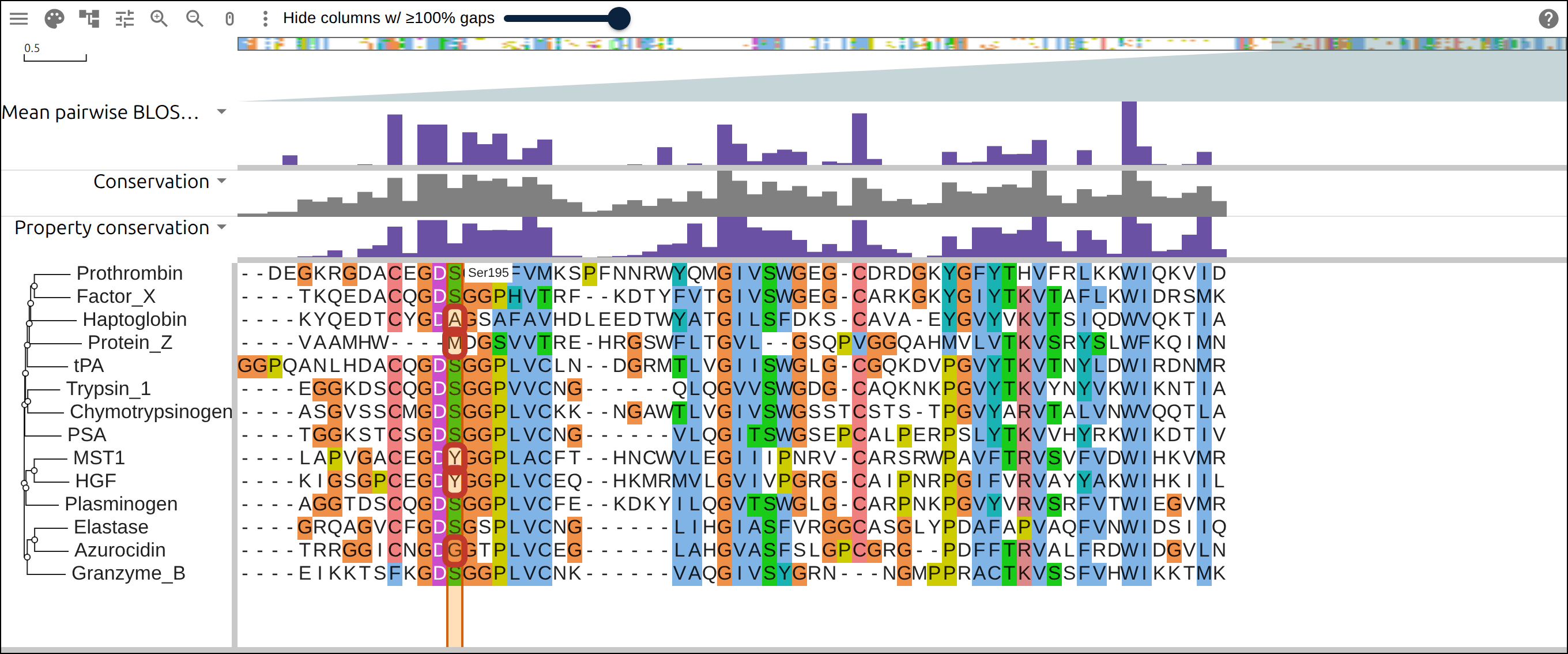
The bands mark three columns of the alignment. Reading them off the matrix takes the same walk the viewer does, one cumulative sum over the reference row:
residue_column <- cumsum(m[ref, ] != "-")
triad_column <- vapply(triad, function(r) which(residue_column == r)[1], integer(1))
data.frame(
  protein = proteins$label,
  charge_relay = ifelse(lengths(proteins$act) > 0, "annotated", "none"),
  His57 = m[, triad_column[1]],
  Asp102 = m[, triad_column[2]],
  Ser195 = m[, triad_column[3]]
)
protein charge_relay His57 Asp102 Ser195
Chymotrypsinogen annotated H D S
Trypsin_1 annotated H D S
Elastase annotated H D S
Granzyme_B annotated H D S
PSA annotated H D S
Prothrombin annotated H D S
Factor_X annotated H D S
Plasminogen annotated H D S
tPA annotated H D S
Haptoglobin none K D A
Azurocidin none S D G
Protein_Z none K D M
HGF none Q D Y
MST1 none Q Q YAll nine active peptidases read H, D and S. Each of the other five reads something else at His57 and at Ser195, and four of them keep the aspartate.
10. Save the widget, or share the link#
saveWidget writes a page that needs no R to open, and the same two layers go
into a URL that opens the hosted alignment in the web viewer:
htmlwidgets::saveWidget(widget, "proteases.html", selfcontained = FALSE)

snapshot <- list(msaview = list(
  type = "MsaView",
  height = 560,
  treeAreaWidth = 150,
  colorSchemeName = "clustalx_protein_dynamic",
  msaFilehandle = list(uri = "data/proteases/proteases.aln"),
  treeFilehandle = list(uri = "data/proteases/proteases.nh"),
  columnTracks = list(blosum_track, ss_track),
  highlights = unname(bands)
))
json <- as.character(jsonlite::toJSON(snapshot, auto_unbox = TRUE, digits = 3))
paste0("https://gmod.org/JBrowseMSA/demo/#data=", URLencode(json, reserved = TRUE))
the link is 3075 charactersunname() matters: Map over a named vector names its result, and a named list
serializes as a JSON object where the viewer reads an array. msaview() drops
the names on the way in, so the widget above works either way.
Reproduce it end to end#
curl -O https://raw.githubusercontent.com/GMOD/JBrowseMSA/main/docs/tutorials/scripts/build_r_protease_triad.R
Rscript build_r_protease_triad.R out/
The script runs every command above and writes out/proteases.aln,
out/proteases.nh, out/proteases-layers.json and out/proteases.html. The
numbers quoted here are the ones it prints.
See also#
- R package, including the Shiny inputs a clicked cell sets
- Data layers
- Influenza drift in a notebook
- A protein family from a list of accessions
References#
- Blow DM, Birktoft JJ, Hartley BS. Role of a buried acid group in the mechanism of action of chymotrypsin. Nature 221:337-340 (1969).
- Rawlings ND, et al. The MEROPS database of proteolytic enzymes, their substrates and inhibitors in 2017. Nucleic Acids Research 46:D624-D632 (2018), which classifies the five rows above as non-peptidase homologues.
- Wright ES. DECIPHER: harnessing local sequence context to improve protein multiple sequence alignment. BMC Bioinformatics 16:322 (2015).
- Paradis E, Schliep K. ape 5.0: an environment for modern phylogenetics and evolutionary analyses in R. Bioinformatics 35:526-528 (2019).
- Henikoff S, Henikoff JG. Amino acid substitution matrices from protein blocks. PNAS 89:10915-10919 (1992).
- The UniProt Consortium. UniProt: the Universal Protein Knowledgebase in 2025. Nucleic Acids Research 53:D609-D617 (2025).