Data layers
Every field below is a property of the MsaView model, so a host can write it
into the standalone app’s #data= URL, pass it to MSAModelF().create, set it
through MSAViewer props, or give it to the R widget. The viewer draws each
layer as given, keeps it in a shared URL, and includes it in the SVG export.
Wherever a layer names a row, positions are that row’s residues, 1-based and
inclusive, as in GFF, and the viewer projects them through the alignment’s gaps.
Without a row, positions are alignment columns.
Every figure below links to the app in the state it shows. Each one is an
MsaView snapshot; to open one, URL-encode the JSON and put it in #data=,
either bare or wrapped as {"msaview": {...}}, the form the app writes back to
the address bar:
const snapshot = {
  type: 'MsaView',
  data: { msa: '>human\nMKAANSE\n>mouse\nMKA-NSE' },
}
const url = `https://gmod.org/JBrowseMSA/demo/#data=${encodeURIComponent(JSON.stringify(snapshot))}`
The user guide covers what else a link needs: file URIs, CORS, and the size limit on inline data.
Shorthand#
A link or a script can write a view in short forms, which expandSpec (exported
from react-msaview) turns into the snapshot. The app’s #data= and
jbrowse-plugin-msaview’s session spec both apply it, and a full snapshot passes
through unchanged.
{
  "type": "MsaView",
  "msa": "https://gmod.org/JBrowseMSA/demo/data/p53/p53-vertebrates.afa",
  "tree": "https://gmod.org/JBrowseMSA/demo/data/p53/p53-vertebrates.nh",
  "query": "Human",
  "highlights": ["102-292 DNA-binding", 175, 248, 273],
  "region": "170-290",
  "columnTracks": [
    {
      "name": "ClinVar",
      "color": "#c0392b",
      "max": 8,
      "start": 104,
      "values": [2, 1, 0, 0, 2, 4]
    }
  ]
}| Short form | Expands to |
|---|---|
msa | msaFilehandle for a url, data.msa for text spanning more than one line |
tree | treeFilehandle for a url, data.tree for newick text starting with ( |
query | relativeTo, and the row of every highlight, region and column track that names none |
a highlight 175 | residue 175 of the query row, labeled with its letter and number, “R175” |
a highlight "102-292 DB" | residues 102-292 labeled “DB”; "248" is residue 248 and "248 hotspot" labels it |
region: "170-290" | {row, start: 170, end: 290} |
a column track’s id | taken from name when absent, “ClinVar pathogenic” becoming clinvar-pathogenic |
a column track’s kind | bar for values, text for data, arc for arcs |
a column track’s start | the position its values or data begins at, so leading zeros stay out of the link |
Without query, the same highlight forms are alignment columns and a single one
gets no label. "row": null on an object entry takes it off the query row onto
alignment columns. A highlight’s label may name {residue} and {position},
which the viewer fills from the row’s letter at start: 175 expands to the
label {residue}{position}. A malformed string, such as "R175" or
"170..290", opens the view on an error naming it.
columnTracks#
A track above the alignment, supplied as data. kind picks what it draws: bar
reads values, text reads data, arc reads arcs. row makes any of them
index that row’s residues instead of alignment columns, so the first one is
residue 1 and the viewer fills in the row’s gaps. A data track appears in the
Tracks menu, toggles like any other, and exports to SVG.
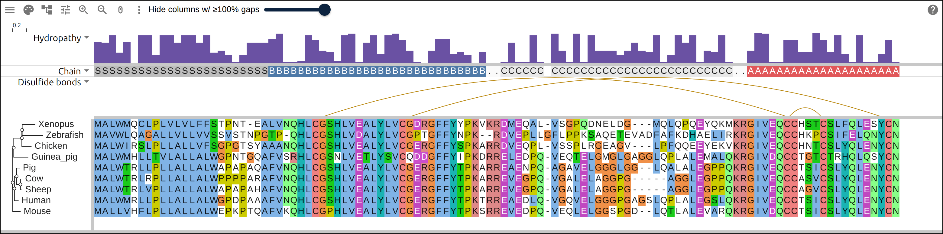
{
  "type": "MsaView",
  "data": { "msa": ">human\nMKAANSE\n>mouse\nMKA-NSE" },
  "columnTracks": [
    {
      "id": "dnds",
      "name": "dN/dS",
      "kind": "bar",
      "values": [0.1, 0.4, 1.8, 0.2, 0.3, 0.1],
      "max": 2,
      "color": "#6a51a3",
      "row": "human"
    },
    {
      "id": "frame",
      "name": "Codon frame",
      "kind": "text",
      "data": "1231231",
      "colors": { "1": "#ddd", "2": "#bbb", "3": "#999" }
    },
    {
      "id": "disulfides",
      "name": "Disulfide bonds",
      "kind": "arc",
      "arcs": [
        { "start": 31, "end": 96 },
        { "start": 43, "end": 109 }
      ],
      "color": "#b8860b",
      "row": "human"
    }
  ]
}| Field | Kind | Meaning |
|---|---|---|
id | both | Unique key. The Tracks menu and turnedOffTracks use it |
name | both | Label beside the track |
values | bar | One number per column, or per residue of row |
max | bar | Value drawn at full height (default 1) |
color | bar | Bar fill (default gray) |
data | text | One character per column, or per residue of row |
colors | text | Upper-case character to background color; the active color scheme otherwise |
arcs | arc | {start, end, color?} pairs; each end is a column or a residue |
row | both | Row name whose residues the values or characters index |
height | both | Pixel height (default 40 for a bar, 50 for an arc, the row height for text) |
A row on an arc track carries both ends of every arc, so a contact map
computed in a protein’s own numbering lands on the alignment without conversion.
The viewer draws arcs on one baseline in the order given, and a color on an
individual arc overrides the track’s, so one track can separate nested helices
from a pseudoknot.
An RNA Stockholm file needs no arc track, because #=GC SS_cons already pairs
the columns. The viewer draws a Base pairs track from it and gives
pseudoknot pairs their own color. WUSS writes a pseudoknot pair as A/a
because it crosses a helix, and brackets can only nest.
A track over 50 kB serialized stays in the live model but leaves the snapshot,
under the same size rule
that applies to inline alignments. The demo app raises the limit to 1 MB, as
much as its links hold, and MSAModelF({ maxInlineSnapshotBytes }) sets it for
another host. To go past it, host the values and set them at runtime with
model.setColumnTracks(...).
highlights#
A labeled band over a column range or a residue range, or a tint over a set of
rows. label and color are optional; color is any CSS color and paints the
band, its border, or the row tint.
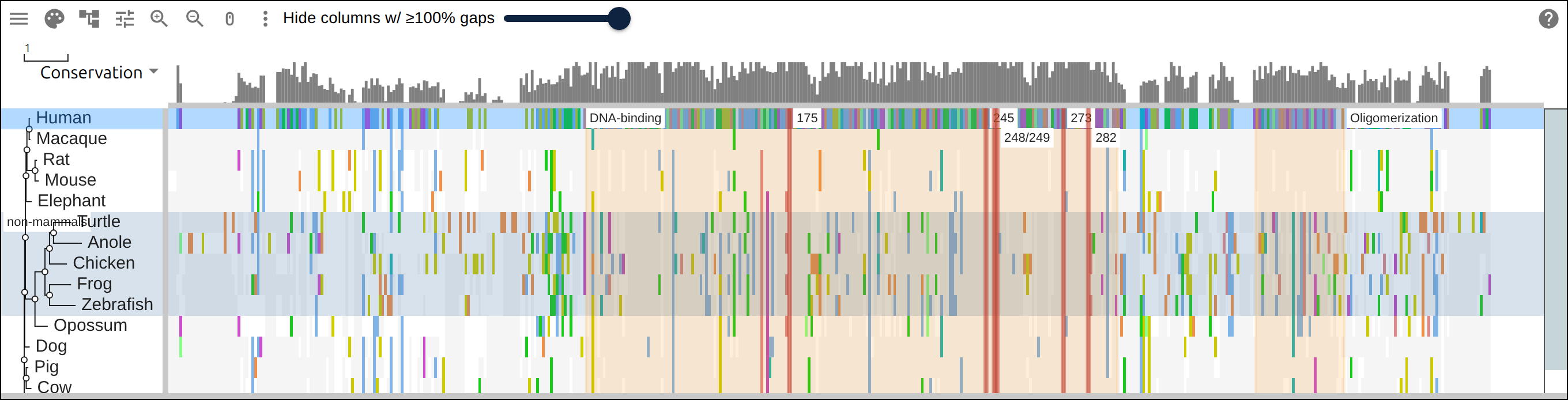
rows entry over the
five non-mammals, labeled in the tree gutter."highlights": [
{ "row": "human", "start": 248, "end": 248, "label": "R248Q · 651/658 R" },
{ "start": 40, "end": 60, "label": "NES", "color": "rgba(0,120,255,0.25)" },
{ "rows": ["beluga", "dolphin"], "label": "frameshift carriers" }
]row plus start/end is a residue range of that row, start/end alone is
a column range, and rows marks whole rows across the tree labels and the
alignment. A range that lands entirely on hidden gappy columns draws nothing;
one that straddles them shrinks to the visible part. The viewer ignores row
names that match no row.
React: the highlights prop on MSAViewer, or model.setHighlights(list). R:
msaview(highlights = list(list(row = "human", start = 248, end = 248))).
For a transient highlight, such as one following a hover in a structure viewer
or a genome browser, call model.applyHighlight(owner, list) and
model.clearHighlight(owner). They take the same shape, draw over the persisted
highlights, and stay out of the snapshot. clearHighlight(owner) removes only
that owner’s highlights, so two sources can highlight at once.
region takes the same coordinates and names where the view opens:
{"row": "Human", "start": 170, "end": 290} zooms onto those residues once the
alignment and any tree file have loaded. The viewer then clears it, so a
reloaded session keeps the reader’s own scroll. model.zoomToRegion(region)
does the same at runtime.
selection#
A block of the alignment, selected: columns start to end of the file,
1-based and inclusive, across the rows rows names, or across every row where
rows is absent. The viewer draws it as a bordered blue band, and a shift-drag
in the viewer replaces it, so a link can open on a block and a script can read
back the block a person chose.
{
  "type": "MsaView",
  "data": { "msa": ">human\nMKAANSE\n>mouse\nMKA-NSE\n>chicken\nMKSANSE" },
  "selection": { "start": 2, "end": 5, "rows": ["human", "mouse"] }
}
Open this snapshot in the app.
start and end count every column of the file, hidden gappy ones included,
the way a column highlight does, so hiding gaps leaves the band on the same
residues. A selection that lies entirely on hidden columns draws nothing. The
header’s selection menu copies the block as FASTA across those columns, gaps
kept, and zooms to it.
React: the selection prop on MSAViewer, with onSelectionChange reporting
each change the reader makes, or model.setSelection(block). R:
msaview(selection = list(start = 2, end = 5, rows = c("human", "mouse"))) or
geom_msa_selection(2, 5, rows = c("human", "mouse")), with
input$<id>_selection in Shiny. Python: the selection trait, which the widget
also writes back.
clades#
A clade of the tree with a mark over it. mark takes one of five values:
highlightfills the rows behind the clade with a translucent rectangle, running from the clade’s common ancestor to the right edge of the tree area and on across the alignment, which is ggtree’sgeom_hilight.bracketdraws a vertical bar beside the clade’s rows carrying the record’slabel, which is ggtree’sgeom_cladelaband, over arange,geom_strip.collapsecollapses the clade at load, the way the branch menu’s “Collapse this node” does.focusopens the viewer on the clade alone, the way “Show only this node” does.rotateswaps the order of the clade’s children at load, the way “Rotate this node” does, which is ggtree’srotate. The rows follow the tips.
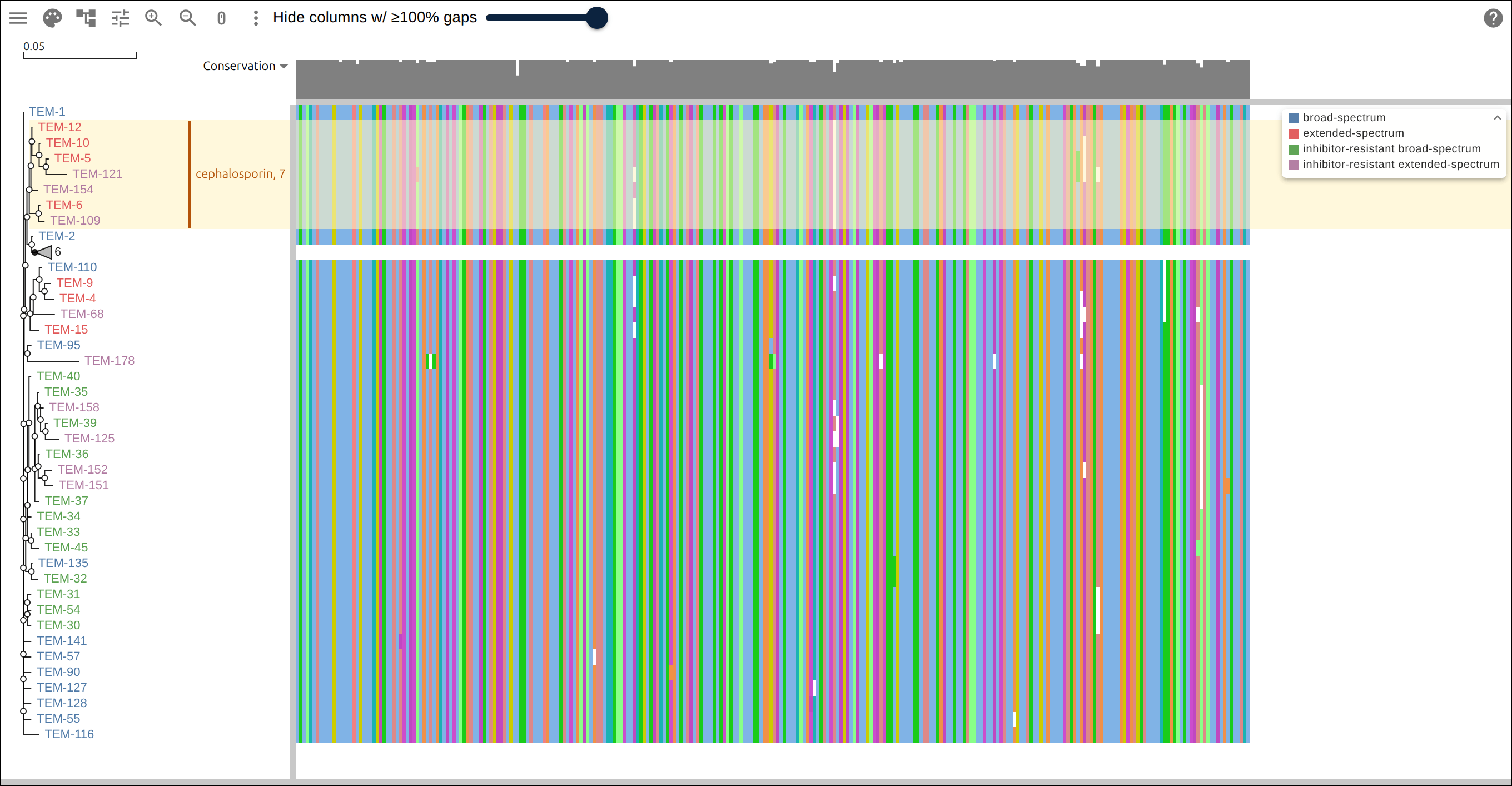
highlight and a bracket over the same mrca; the clade under it carries a
collapse and draws as a triangle labeled with its six tips. Tip labels take
their color from an encodings entry over the phenotype field."clades": [
{
"mrca": ["Gs/TW/TNC1/2015", "Ck/TW/a174/2015"],
"tips": 47,
"mark": "highlight",
"color": "#fff3c4",
"label": "2.3.4.4 H5Nx"
},
{
"mrca": ["Gs/TW/TNC1/2015", "Ck/TW/a174/2015"],
"tips": 47,
"mark": "bracket",
"color": "#b45309",
"label": "2.3.4.4 H5Nx"
},
{ "mrca": ["Dk/VN/1/2012", "Ck/VN/14/2012"], "tips": 6, "mark": "collapse" }
]mrca names tips whose most recent common ancestor is the clade, and the mark
covers every tip under that ancestor. Two names are enough for a clade of any
size, and a name the tree does not have, or has twice, drops the record.
tips is the leaf count the producer measured. The viewer counts the leaves
under the ancestor it resolved, and a count that differs drops the clade, so a
re-rooted or re-estimated tree loses the mark instead of drawing it over a
different clade.
range takes the two ends of a run of tips in display order, in either order,
and covers every tip between them, monophyletic or not. Its tips is checked
against the length of the run:
{ "range": ["Dk/VN/1/2012", "Ck/VN/14/2012"], "tips": 6, "mark": "highlight" }color is any CSS color, defaulting to a light yellow. A highlight’s color
carrying no alpha of its own draws at 60% opacity, so the branches and the
residues under it stay readable. A bracket draws its bar and its label in that
color at full strength, and takes the theme’s text color without one.
The bracket gutter is at the right of the tree area, between the tip labels and
the first row panel or the alignment, as wide as the bar plus the widest label
at the tree font, to a limit of 140px, past which a label is cut with an
ellipsis. A label reads across the rows where they are taller than the font, and
runs up the bar where they are not. A highlight record carrying a label
draws it the same way, with no bar.
collapse, focus and rotate seed the viewer’s own collapsed, showOnly
and rotated lists when the tree resolves, so hideGaps counts the rows that
remain exactly as when the user collapses a clade by hand. The three marks name
a node, so they need mrca: a range record carrying one of them drops.
Expanding a seeded clade or clearing the focus holds until the tree is rerooted,
and the record applies again the next time the link is opened.
Every mark resolves against the tree as loaded, so collapsing a clade’s ancestor or focusing on part of the tree keeps the mark on the rows that remain on screen.
React: the clades prop on MSAViewer, or model.setClades(list). R:
geom_msa_clade(c("Gs/TW/TNC1/2015", "Ck/TW/a174/2015"), tips = 47).
treeOrder and treeRoot#
treeOrder sets the order each node’s children draw in, top to bottom, and the
rows of the alignment follow the tips:
branchLength, the default, puts the child with the shorter branch first.inputkeeps the order the tree file gives.ladderizeputs the child with fewer tips first, so the deep clades step down toward the bottom, which is ape’sladderizeasplot.phylodraws it.ladderizeReverseputs the child with more tips first, which is ggtree’s default.
A rotation from the branch menu or a rotate clade reverses one node’s children
after the order applies. “Undo rotations” in the tree settings clears them.
treeRoot reroots the tree before the viewer draws it. "midpoint" puts the
root halfway along the longest path between two tips, the usual root for the
unrooted trees FastTree, IQ-TREE and neighbor joining write. An outgroup puts it
halfway along the branch above the tips’ most recent common ancestor:
"treeRoot": { "outgroup": ["Dk/VN/1/2012", "Ck/VN/14/2012"] }Where that ancestor is the root of the file’s tree, the outgroup straddles the root, and the viewer roots above the common ancestor of the other tips, which is the same branch of the unrooted tree. A tree whose outgroup resolves to neither side, or names a tip it does not have, keeps its own root.
A support value labels the branch above its node. When the viewer reroots, the nodes between the new root and the old one turn over, and each support value moves with its branch to the node now at the lower end of it. A root with two children has one branch left once the new root takes one of them, so the viewer drops it and joins its two branches into one.
“Reroot here” in the branch menu writes the outgroup as the first and last tip
of the node’s side of the split in the file’s tree, so a second reroot resolves
against the file and the link stays short. Rerooting renumbers the nodes, so it
clears collapsed, rotated and showOnly, and the collapse, focus and
rotate clades seed again on the new tree.
React: the treeOrder and treeRoot props on MSAViewer, or
model.setTreeOrder(order) and model.setTreeRoot(root). R:
coord_tree(order = "ladderize", root = "midpoint"), or root as a vector of
outgroup tip names. Python: tree_order and tree_root, the latter
"midpoint", one tip name or a list of them.
rowData#
A table of fields per row, keyed by row name: a lineage, a host, a collection
date, a kinase group. The encodings below color the viewer’s marks by one of
these fields, the tree’s node-info dialog lists a row’s fields, and a genome
field replaces the row name in the tree labels.
The model keeps the table as the JSON string data.treeMetadata, the field name
that travels in existing links, so a snapshot carries it there:
{
  "type": "MsaView",
  "data": {
    "msa": ">duck\nMKAANSE\n>chicken\nMKA-NSE",
    "treeMetadata": "{\"duck\":{\"clade\":\"2.3.4.4b\"},\"chicken\":{\"clade\":\"2.3.2.1c\"}}"
  }
}
Open this snapshot in the app.
Everywhere else the table is an object: the rowData prop on MSAViewer,
model.setRowData(table), geom_msa_rowdata(df) in R, and the row_data trait
in Python. R takes a data frame whose label or row column names each row and
whose other columns are the fields, the shape a ggtree
tibble(label = , trait = ) has.
A field’s value can be a string, a number or a boolean. The viewer reads a
number or a boolean as its string, 2015 as "2015", the way it reads a GFF
attribute, and leaves out a null or a nested object.
A real metadata table needs the filehandle. Five thousand rows with eight fields
run to roughly 700 kB, far past the 50 kB inline limit a jbrowse session keeps,
so the snapshot drops the table and unshareableData reports the drop. Host the
JSON and set treeMetadataFilehandle to its URL, and the viewer fetches the
table at startup:
{
  "type": "MsaView",
  "msaFilehandle": { "uri": "https://example.org/h5.fa" },
  "treeMetadataFilehandle": { "uri": "https://example.org/h5-lineages.json" }
}features#
Features on the rows as JSON, the form a GFF line takes once parsed: row,
start and end in residues of that row, 1-based and inclusive, with an
optional name, description, type, strand and color. The viewer draws
them in the annotation overlay beside the GFF’s, under the same legend, filter
dialog and feature channels.
{
  "type": "MsaView",
  "data": { "msa": ">human\nMKAANSEMKAANSE\n>mouse\nMKA-NSEMKA-NSE" },
  "features": [
    { "row": "human", "start": 2, "end": 7, "name": "SH3", "source": "pfam" },
    { "row": "mouse", "start": 3, "end": 9, "name": "SH2", "source": "smart" }
  ],
  "encodings": [{ "channel": "featureFill", "field": "source" }]
}
Open this snapshot in the app.
name is the key the legend, the accession palette and the filter dialog group
features by, and an unnamed feature takes row:start-end. color overrides the
palette and any scale, as a GFF color= attribute does. A strand of + or
- draws the span as an arrow whatever its type, and a type of exon,
CDS or a UTR draws it as a numbered segment. Every other field, such as
source above, is a column the featureFill and featureLabel channels read
the way they read a GFF attribute.
A host that computes its spans passes them here, and a file of them loads
through data.gff or gffFilehandle. React: the features prop on
MSAViewer, or model.setFeatures(features). R: a data frame given to
msaview(gff = ) or geom_msa_domains(), with a row (or seqname) column
and every other column a field. Python: the features trait, which takes a list
of dicts or a DataFrame.
encodings#
What the viewer’s own marks read from a table. Each entry names a channel, the
field feeding it, and the scale that turns a field value into a color.
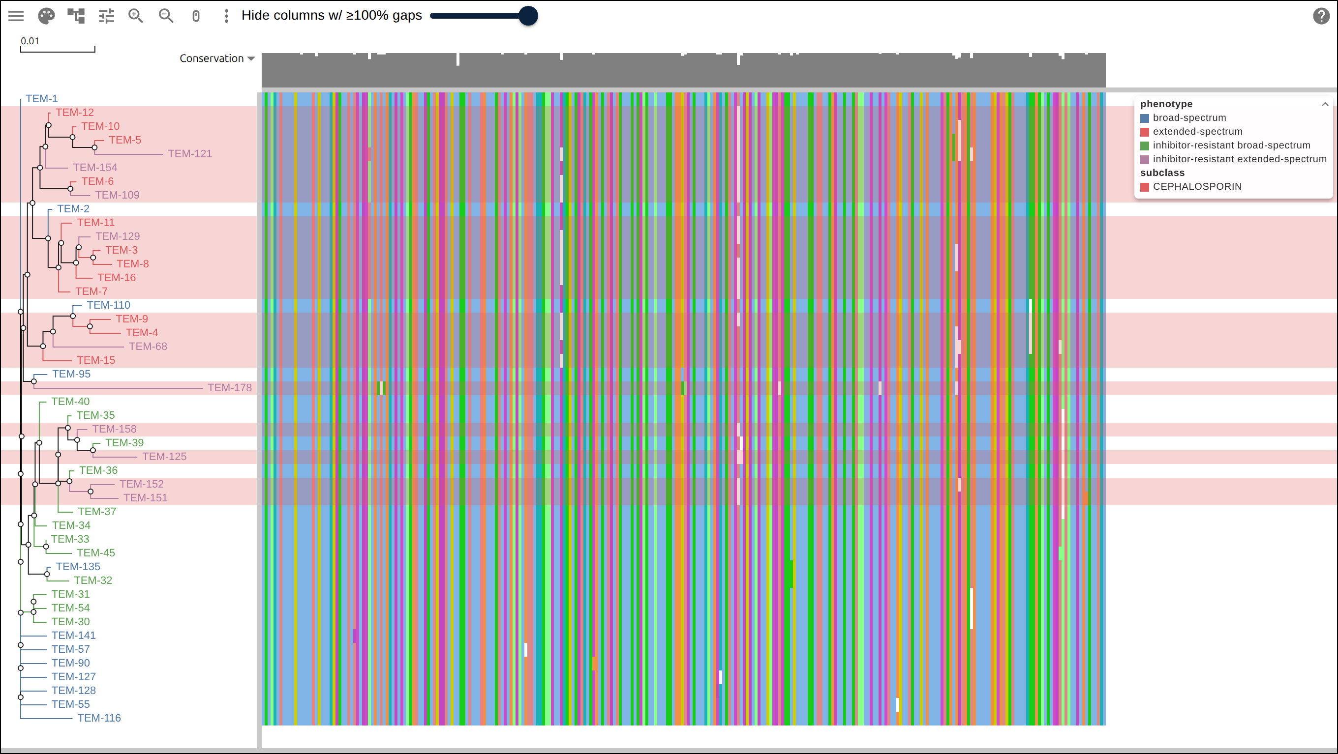
tipLabel and
branch over the phenotype field, and rowTint over the subclass field through
a {map} that names one of its two values, so the alleles it leaves out take no
tint. Each field lists its own legend.{
"type": "MsaView",
"data": { "msa": ">duck\nMKAANSE\n>chicken\nMKA-NSE" },
"encodings": [
{ "channel": "tipLabel", "field": "clade", "scale": { "palette": "set1" } },
{
"channel": "rowTint",
"field": "clade",
"scale": { "map": { "2.3.4.4b": "#e41a1c" } }
}
]
}| Field | Meaning |
|---|---|
channel | one of the five below |
field | the field the channel reads |
scale | {palette} or {map}; the ggplot palette when the entry omits it |
| Channel | What it sets | Reads a field of |
|---|---|---|
tipLabel | the color of each tip label in the tree | rowData |
rowTint | a wash over the row, across the tree gutter and the alignment | rowData |
branch | the color of a tree edge whose tips all share one value | rowData |
featureFill | the fill of each span of the annotation overlay | the gff |
featureLabel | the text drawn inside a span | the gff |
A {palette} names one of ggplot (the default), set1, dark2, okabeito
and tableau, and the scale hands its colors to the field’s distinct values in
sorted order, so a value keeps its color as rows are collapsed, filtered or
re-ordered. Past the end of a palette every value takes an evenly spaced hue
instead, which keeps a forty-clade field readable. A {map} names a color per
value, and a value it leaves out keeps the plain mark: an uncolored tip label
draws in the theme’s text color, an uncolored row takes no tint, and an
uncolored span draws grey.
A tint draws at 25% opacity so the residues under it stay readable. A color
carrying its own alpha, such as rgba(228,26,28,0.5), draws at that alpha.
The branch channel gives an internal node the field’s value when every tip
below it shares that value, and that node’s edge and every edge inside the clade
draw in the scale’s color for it. An edge whose tips disagree draws in the
default color, and a collapsed clade’s triangle takes the color of the value its
tips agree on. This is ggtree’s groupClade followed by aes(color = group),
with the group read from the table.
Every field an encoding reads carries a legend of its scale, titled by the field name, drawn by the overlay on screen and reserved as a column in the SVG export. Two channels over one field list that field once.
The feature channels#
A feature channel reads any field of the feature table: accession, name,
featureType, any GFF attribute of column 9, such as Name or gene, or any
field of a features record.
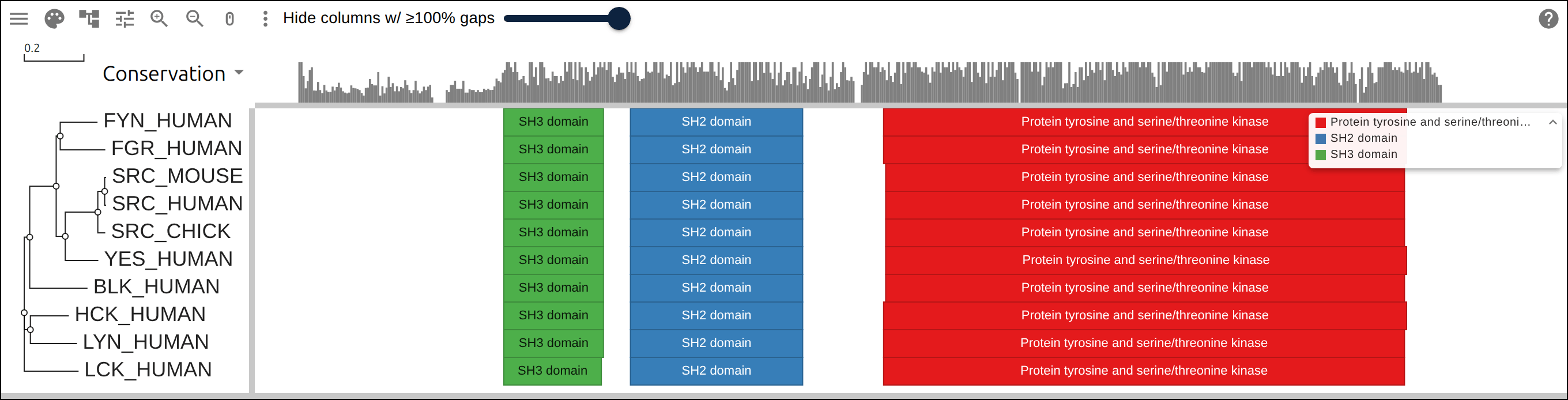
description attribute: featureFill colors each span from a
set1 scale and featureLabel draws the same value inside it.{
"type": "MsaView",
"data": {
"msa": ">duck\nMKAANSE\n>chicken\nMKA-NSE",
"gff": "##gff-version 3\nduck\tncbi\tgene\t1\t5\t.\t+\t.\tName=HA;class=surface\nchicken\tncbi\tgene\t1\t4\t.\t+\t.\tName=NP;class=internal;color=255,0,0"
},
"encodings": [
{
"channel": "featureFill",
"field": "class",
"scale": { "palette": "set1" }
},
{ "channel": "featureLabel", "field": "Name" }
]
}The featureFill scale replaces the accession palette the overlay colors spans
by, so a span whose value the scale gives no color draws grey, and the domain
legend lists that scale’s values under the field’s name. A feature carrying a
GFF3 color= attribute keeps that color whatever the scale says, and 255,0,0
reads as rgb(255,0,0), the convention JBrowse and IGV honor. A featureLabel
draws inside its span wherever the text fits, and it is a data channel, so it
draws whether or not the residue letters do.
customColorScheme#
A color per residue letter, which replaces the built-in color scheme while it is
set. The letters the map lists take its colors, and every other letter is
uncolored, the rule a {map} scale in encodings follows.
{
  "type": "MsaView",
  "data": { "msa": ">human\nMKAANSE\n>mouse\nMKA-NSE" },
  "customColorScheme": {
    "K": "#1f77b4",
    "R": "#1f77b4",
    "D": "#d62728",
    "E": "#d62728"
  }
}
Open this snapshot in the app.
The viewer upper-cases every row before coloring it, as the built-in schemes
expect, so a key matches its letter in either case. A gap is uncolored unless
the map lists - or .. The map paints whichever channel residueEncoding
picks, the cell or the letter, and it colors the sequence logo’s letters too.
Picking a scheme from the palette menu clears the map.
React: colorScheme={{ map: { K: '#1f77b4' } }} on MSAViewer, or
model.setCustomColorScheme(map). R: color_scheme = c(K = "#1f77b4"), or
scale_residue_color(c(K = "#1f77b4")). Python:
color_scheme={"K": "#1f77b4"}.
rowPanels#
A panel beside the tree on the row scale, the counterpart of columnTracks on
the column scale. Each record names a kind. A strip reads a field of
rowData and colors each row’s cell through scale, and eight strips make the
tip-aligned matrix ggtree draws with gheatmap. A features panel draws the
spans gff carries, one row per alignment row, which is gggenes.
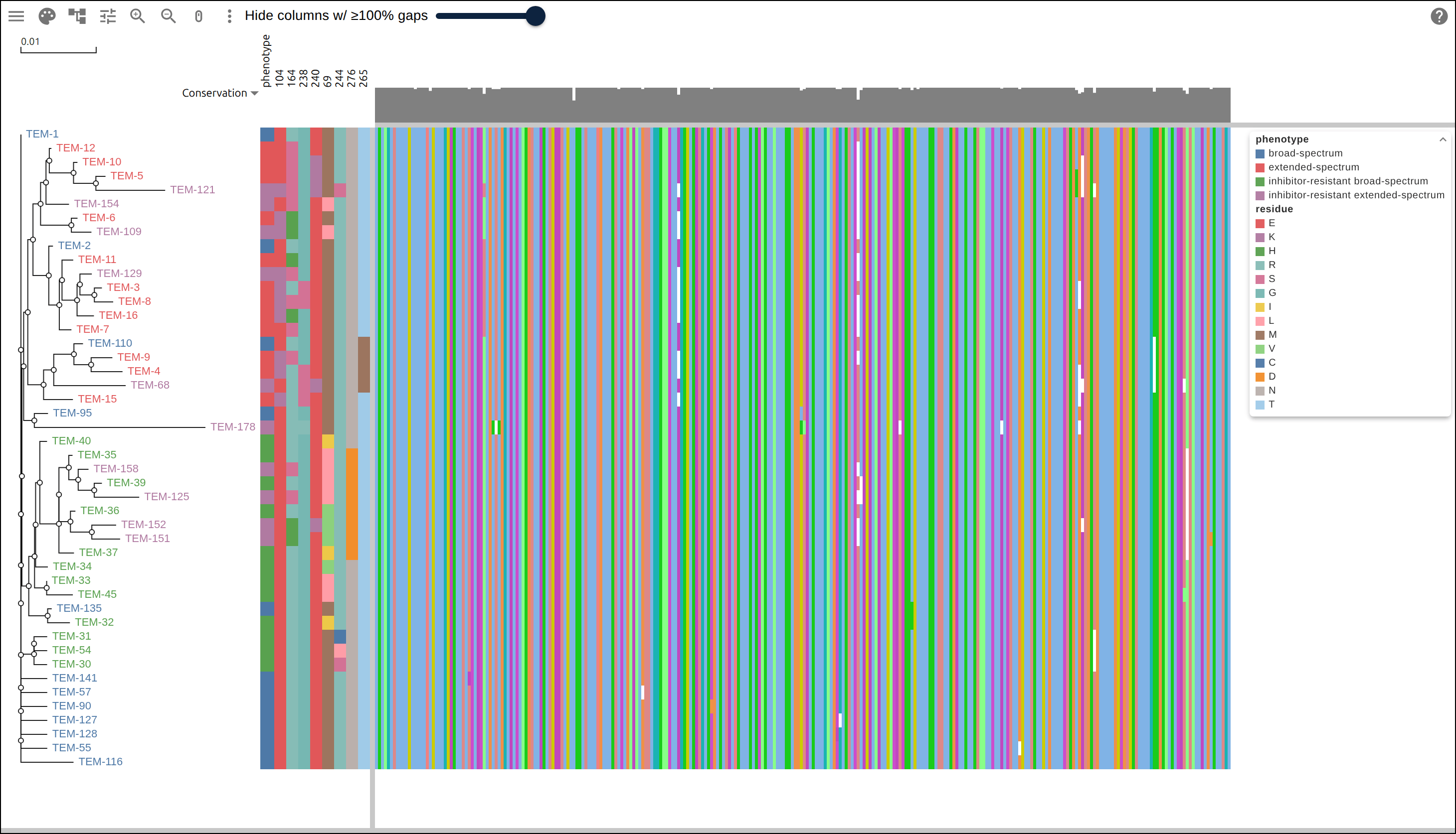
legend, so the matrix carries a single key for its
residue colors.{
"type": "MsaView",
"data": {
"msa": ">duck\nMKAANSE\n>chicken\nMKA-NSE",
"treeMetadata": "{\"duck\":{\"HA\":\"H5\",\"NA\":\"N1\"},\"chicken\":{\"HA\":\"H5\",\"NA\":\"N8\"}}"
},
"rowPanels": [
{
"kind": "strip",
"field": "HA",
"scale": { "palette": "set1" },
"width": 12
},
{ "kind": "strip", "field": "NA", "header": "NA segment" }
]
}| Field | Meaning |
|---|---|
kind | strip or features |
field | the rowData field a strip’s cells read |
scale | {palette} or {map}; the ggplot palette when the record omits it |
width | the column’s pixel width: a row height for a strip, 200 for features |
header | the name drawn above the column, defaulting to a strip’s field |
legend | the title a strip’s values list under, defaulting to its field |
The panels take their width out of the alignment’s, so the alignment scrolls and fits within what is left. A strip scrolls with the tree and the alignment, and a row the table gives no value leaves its cell empty.
Each header draws in the band the tree’s scale bar and the minimap share, turned on its side, and it exports with the figure. The band is as tall as the minimap, so a longer header is clipped to it and the full name is the column’s tooltip.
A panel’s scale carries a legend of its own, titled by the field, and every
panel and encoding over one field lists that field once. Eight columns over one
set of colors read eight fields, so give them one legend and the figure
carries one key for the matrix:
"rowPanels": [
  { "kind": "strip", "field": "PB2", "scale": { "map": { "am2.2": "#4e79a7" } }, "legend": "segment lineage" },
  { "kind": "strip", "field": "PB1", "scale": { "map": { "am4": "#f28e2b" } }, "legend": "segment lineage" }
]
A features panel taking the overlay’s colors lists them under the same key the
overlay draws, and with no alignment behind it the panel’s own entries are that
key.
React: the rowPanels prop on MSAViewer, or model.setRowPanels(list). R:
geom_msa_strip("HA", palette = "set1", width = 12, legend = "amino acid") and
geom_msa_features(color = "Name", label = "Name", align = "genE"). Python: the
row_panels trait.
The features panel#
A features record draws the same spans the alignment’s overlay draws, in a
column of its own: an arrow where the GFF gives a gene a strand, a box
otherwise, labeled where the text fits. Features that overlap within a row stack
into lanes, which divide the row’s height between them.
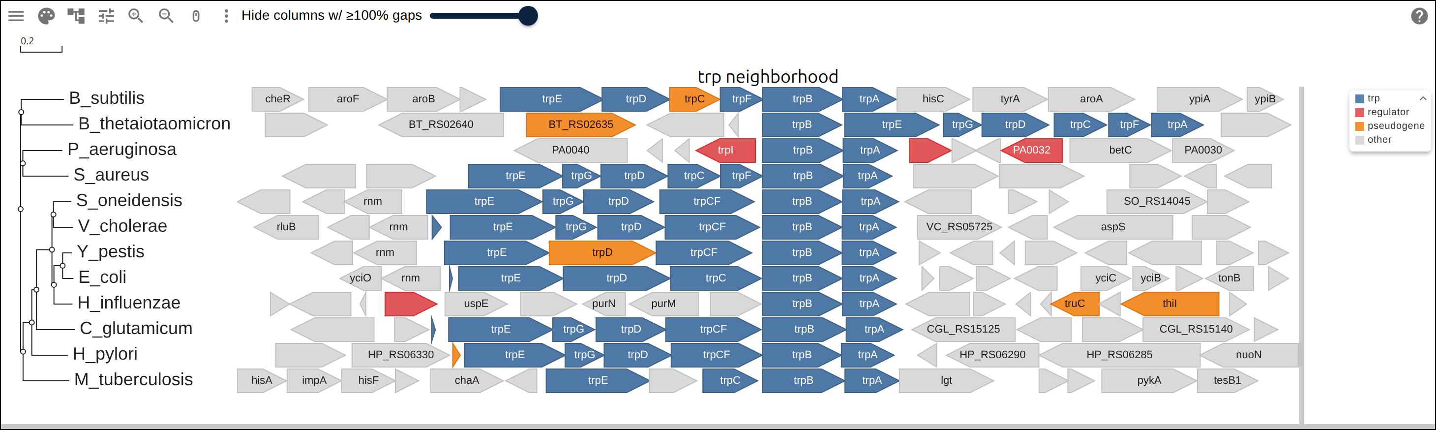
trpB, with no alignment at all: a tree, a GFF
and one features panel under x: "position". The align transform starts
trpB at one x down the panel, and encoding.color reads the GFF’s role
attribute while encoding.label reads Name.| Field | Meaning |
|---|---|
x | column draws in the alignment’s columns; position in each row’s own residue positions |
encoding | {color: {field, scale}, label: field} over a field of the features |
transform | [{type: "align", on: <Name value>}], only under x: "position" |
position | identity stacks overlapping features; strandpile splits the row by strand |
x: "position" maps every row’s features onto one linear scale across the
extent they cover, so a genome with no alignment has an x. With no msa the
alignment panel is zero columns wide, and the tree and the panel fill the view.
{type: "align", on: "genE"} shifts each row so that the first feature whose
Name is genE starts at zero, which is gggenes’ make_alignment_dummies. A
row carrying no such feature keeps its own origin. An align under
x: "column" draws nothing different, since the columns are the alignment’s.
encoding.color reads any field of the feature table, the same fields a
featureFill encoding reads. A record naming none takes the colors the overlay
gives the same features, and encoding.label falls back to the featureLabel
encoding the same way. A feature’s own GFF color= wins over either.
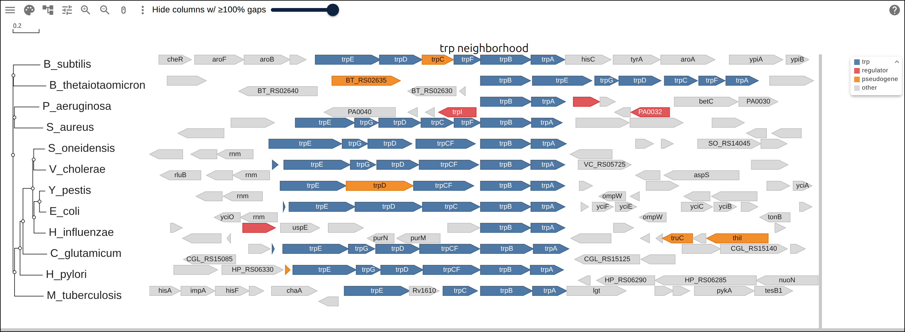
position: "strandpile", which separates the divergently
transcribed neighbours that read as one more arrow in a row under identity.position: "strandpile" is gggenomes’ position_strandpile. Each strand packs
on its own, and the deepest row on each side sets the grid every row lays out
on, so the line between the strands sits at one height down the panel. A row
using only one side leaves the other empty, and a feature with no strand piles
with the forward ones.
{
  "type": "MsaView",
  "data": {
    "tree": "((genome1:0.1,genome2:0.1):0.2,genome3:0.3);",
    "gff": "##gff-version 3\ngenome1\tncbi\tgene\t1\t500\t.\t+\t.\tName=genD\ngenome1\tncbi\tgene\t600\t1000\t.\t+\t.\tName=genE\ngenome2\tncbi\tgene\t200\t700\t.\t+\t.\tName=genE\ngenome3\tncbi\tgene\t1\t400\t.\t-\t.\tName=genD"
  },
  "rowPanels": [
    {
      "kind": "features",
      "x": "position",
      "width": 320,
      "header": "neighborhood",
      "encoding": {
        "color": { "field": "Name", "scale": { "palette": "set1" } },
        "label": "Name"
      },
      "transform": [{ "type": "align", "on": "genE" }]
    }
  ]
}residueMappings#
A residue mapping records which residue of which structure each residue of a row
corresponds to. Unlike the layers above, residueMappings draws nothing; the
model reads it to answer lookups. The host has to supply it, because matching a
row to a structure by sequence equality fails for a construct with an expression
tag, a truncation, an engineered residue, or a row that is a subsequence of the
entry. The highlight then lands on a real residue, just the wrong one. A
producer such as SIFTS, an AlphaFold model or a curator computes the
correspondence.
"residueMappings": [
  {
    "row": "HBA_HUMAN/1-142",
    "accession": "P69905",
    "structure": {
      "id": "1A3N",
      "kind": "experimental",
      "asymId": "A",
      "url": "https://files.rcsb.org/download/1A3N.cif"
    },
    "segments": [
      { "rowStart": 1, "rowEnd": 141, "structStart": 2, "structEnd": 142 }
    ],
    "unobserved": [[60, 62]],
    "rowLength": 142,
    "generated": { "by": "sifts", "date": "2026-09-10" }
  }
]| Field | Meaning |
|---|---|
row | The alignment row this maps |
accession | The sequence database entry the mapping went through, for provenance |
structure | id, plus optional kind, asymId (the chain) and url |
segments | Contiguous runs where the two sides line up 1:1 |
unobserved | Structure positions declared but not resolved, as [start, end] |
rowLength | Ungapped length of the row it was computed against; always set it |
generated | Who computed it, when, and from what |
Positions are 1-based and inclusive on both sides, as everywhere else in this
document. Structure positions are label_seq_id, the index into the entity’s
SEQRES. Author numbering carries insertion codes, which break integer
arithmetic, so the layer does not use it.
A mapping is a few contiguous runs, and the segments define what is unmapped, so the layer needs no status field that could contradict them. A position is in one of three states:
- covered by a segment and not in
unobserved: mapped and observed - covered and listed in
unobserved: mapped, not observed - anything else: unmapped
The middle state separates “the crystallographer could not see this residue” from “this protein has no such residue”.
Two model methods read it:
model.structureResidue(rowName, seqPos, structureId?) // -> {structure, position, observed} | undefined
model.rowResidue(structureId, position, asymId?) // -> {rowName, seqPos} | undefined
Both return undefined when no mapping covers the position, and also when
more than one does. A row commonly maps onto several structures, such as an
experimental entry and a couple of predicted models, and a homodimer maps two
rows onto two chains of one id. Returning the first mapping found would place
the answer on a wrong residue with no error. Name one structure or chain with
the optional argument, or read mappedStructures to see what is available.
Staleness#
A host can load a saved mapping against a re-aligned, revised or different sequence, and every lookup would then return a wrong residue with no error. Before answering, the viewer checks each mapping and stops using it when any of these holds:
- The row it names is not in the alignment.
rowLengthis declared and does not match the row’s ungapped length. No other check catches a same-length substitution, so a producer should always set it.- A segment covers residues past the end of the row, which shows the same
mismatch when
rowLengthis missing.
When a segment is malformed, its two sides differing in length so it cannot be a 1:1 run, the viewer drops only that segment and keeps using the rest of the mapping.
model.residueMappingProblems lists each mapping or segment the viewer dropped,
with a scope (mapping or segment) and a reason, so a host can tell “there
is no structure for this row” from “this data no longer matches what is loaded”.
model.usableResidueMappings holds the mappings that passed.
packages/examples/src/examples/kinaseStructure.json is a real mapping,
generated by scripts/examples-gen/contacts.mjs from SIFTS: the SRC_HUMAN row
against chain A of 2SRC, one segment putting row residue 86 at structure residue
2, one unobserved range, and rowLength: 536. The
spike_structure tutorial
builds another from scratch, against a construct whose numbering is offset by 19
and whose furin loop has no coordinates at all.
seqPos is 1-based, like the rest of this document, and composes directly with
applyHighlight. The column helpers on the model (seqPosToVisibleCol) take
0-based positions, so a structure hover reaches a column as
model.seqPosToVisibleCol(rowName, seqPos - 1).
Generating a mapping#
react-msaview-cli residue-mappings writes this layer from SIFTS for a PDB
chain, or from AlphaFold DB for a predicted model. It checks each row against
its UniProt sequence first, maps a /start-end row as that fragment, and sets
rowLength, unobserved and generated. The
CLI README
lists its options.
react-msaview-cli residue-mappings --msa spike.afa --row SARS-CoV-2 \
  --accession P0DTC2 --pdb 6VXX --chain A -o mappings.json