JBrowseMSA user guide
JBrowseMSA (the react-msaview package) renders a phylogenetic tree alongside a
protein or nucleotide alignment on HTML5 canvas, tiled so it stays responsive on
very large inputs (up to the 230k-node UCSC SARS-CoV-2 sample tree). The viewer
runs entirely in the browser and uploads nothing.
This guide tours the live app. Every
figure below links to the app in that exact state through the #data= URL
fragment, so clicking a screenshot opens the same view to explore.
Getting started#
Open the app and you land on the import form.
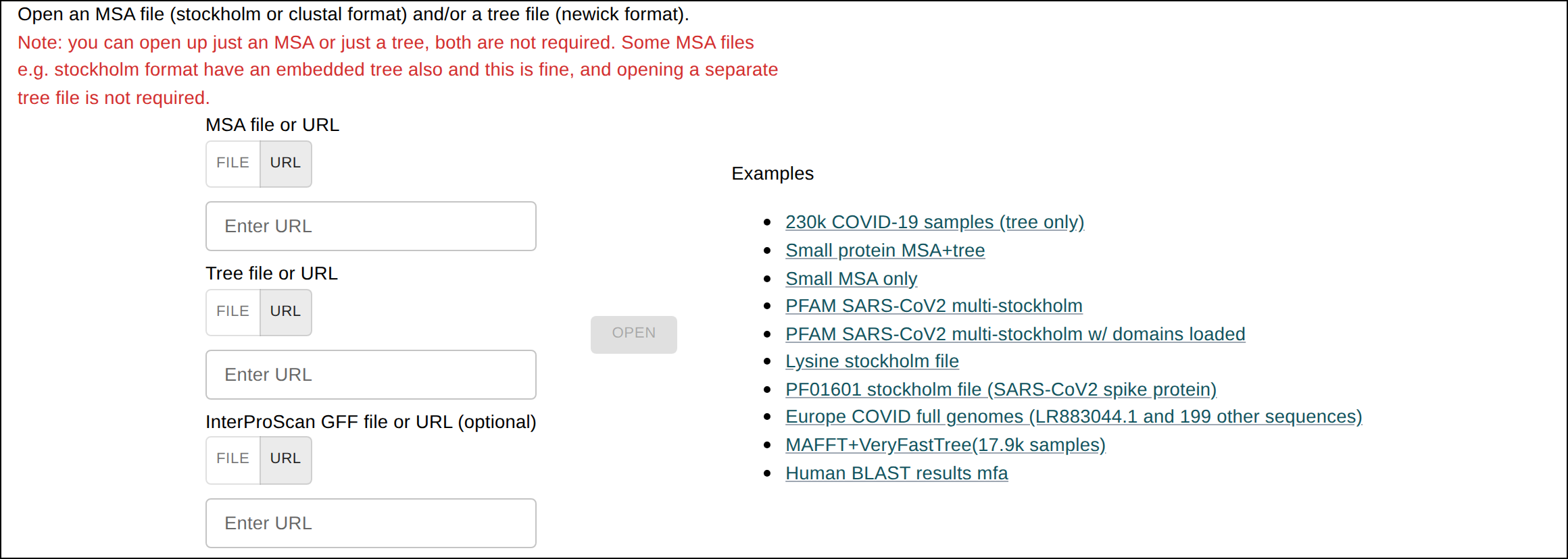
You can load an alignment on its own, a tree on its own, or both together. When both are present, rows are ordered and connected to match the tree.
Loading your own data#
The import form accepts a local file or a remote URL for each of the alignment, the tree, and (optionally) a domain-annotation track. If you do not have those files yet, the tutorials build them from sequences, with the commands for the alignment, the tree and the annotations.
| Input | Formats |
|---|---|
| Alignment | FASTA (gaps already inserted), Stockholm (.stock, single or multi-alignment, may embed a tree and SS), Clustal (.aln), A3M, EMF |
| Tree | Newick (.nh), or the tree embedded in a Stockholm/EMF file |
| Domains | GFF3, such as InterProScan output (generate it with the CLI) |
Stockholm files may carry both the tree and a secondary-structure annotation inline, so a single file can populate the whole view. A “multi-Stockholm” file with several alignments is supported too.
A tour of the viewer#
Once data is loaded the view has four parts:
- Tree panel (left): the phylogeny, with clickable branch nodes.
- Alignment panel (right): the residues, colored by the active scheme.
- Header (top): menu buttons for files, color schemes, and tree/MSA settings, plus zoom controls.
- Minimap & tracks: an overview ruler above the alignment for navigation, and a strip of per-column tracks sharing the alignment’s columns (see Tracks).
Hovering a column highlights that position down every row of the alignment, so you can read one site down the whole family.
Navigating#
- Pan by click-dragging the alignment, or scroll vertically/horizontally.
- Go to a row, a column or a residue from the box in the header: a row name,
which completes as you type, a column number as the ruler reads it, or
name:Nfor residue N of that row. The view centers on the target and lights it, and an entry that names nothing turns the box red. - Keyboard: click the alignment, then the arrow keys move one cell (a page
with shift),
+and-zoom, and Home and End jump to the first and last column. - Select a block of cells by holding shift and dragging across the
alignment, or a range of columns across every row by dragging along a track,
such as the Position ruler. The header then shows the block’s size, such as
“12 columns × 3 rows”, as a button whose menu copies the block as FASTA, zooms
to it, or clears it. Escape clears it too. The selection travels in the
#data=link. - Zoom with the magnifier buttons in the header. Ctrl+wheel zooms at the cursor whatever the wheel is set to do.
- Mouse wheel: the mouse button in the header opens a menu with the four things the plain wheel can do: scroll the alignment, zoom both axes, zoom columns only, or zoom rows only. Zooming columns only holds the row height, so the labels stay at their size while the alignment compresses; rows only holds the column width. The button’s icon shows the mode in force. Hold shift to pan while the wheel zooms.
- Fit the alignment to the window on both axes, horizontally or vertically from the zoom controls. Reset zoom returns to the defaults.
- Set a small row height and column width to zoom out far enough to see a whole large alignment at once.
Color schemes#
Open the palette menu in the header to switch schemes live.
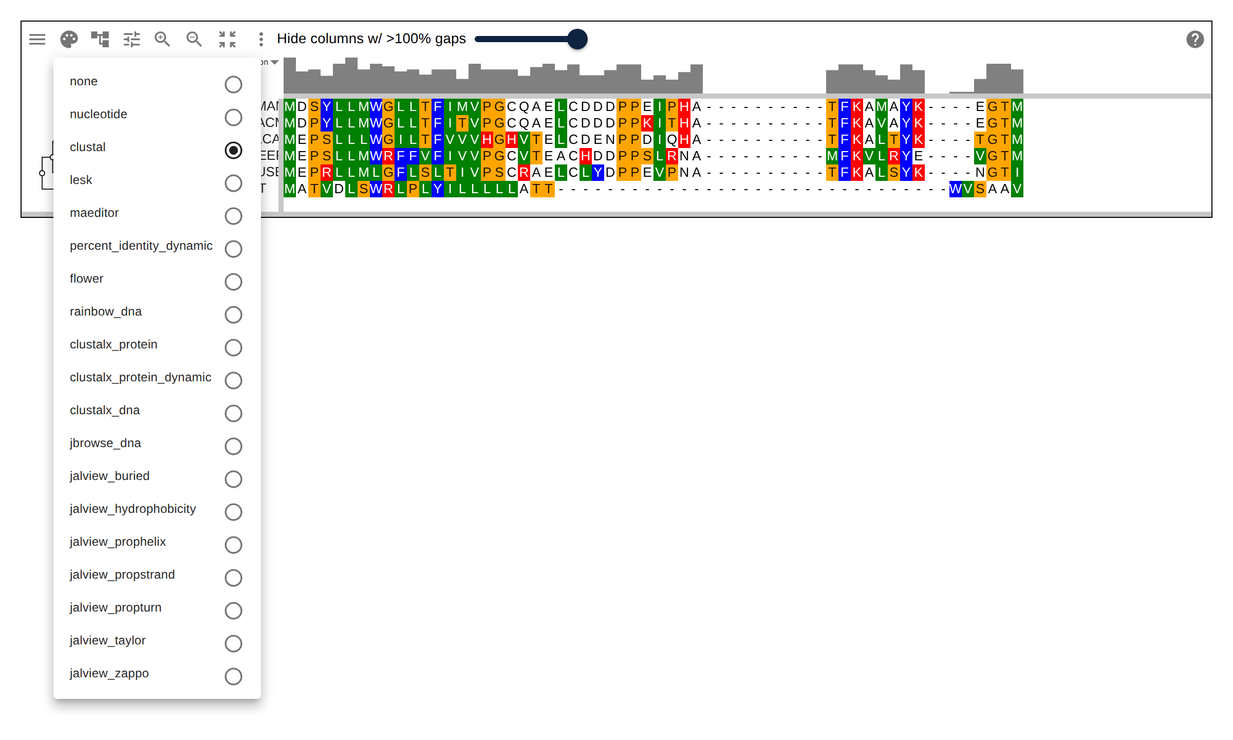
Two schemes are dynamic: they color each column from statistics about the residues in that column, where the other schemes use a fixed color per letter.

clustalx_protein_dynamic colors residues ClustalX-style from the composition
of each column.
percent_identity_dynamic shades each column by its percent identity, so
conserved sites stand out.A link can also color letters from its own map of residue letter to color. The menu then shows a checked Custom entry, and picking a scheme replaces the map.
Working with the tree#
Click a branch node to collapse that subtree. Collapsing also hides any alignment column that holds only gaps once the collapsed rows are gone, so the alignment narrows as you fold clades away.

A branch node’s menu also has Show only this node, which narrows the view to that subtree: the rows below it are the whole alignment until Disable show only this node puts the rest back.
Rotate this node swaps the clades below a branch node, the way ggtree’s
rotate does, and the alignment rows move with the tips. A second click puts
them back, and Tree settings → Order → Undo rotations clears every rotation.
The same Order submenu sets the child order for the whole tree: by branch length
(the default), as the file writes it, or ladderized with the small or the large
clades first.
Reroot here, on any node but the root, roots the tree halfway along the
branch above that node. Tree settings → Root → Midpoint roots it halfway
along the longest path between two tips, which suits the unrooted trees
FastTree, IQ-TREE and neighbor joining write. Rerooting renumbers the nodes, so
it expands collapsed clades, clears rotations and leaves the show-only view.
File → Export tree (Newick) saves the tree with the root, order and
rotations on screen, collapsed clades included.
Data layers covers
treeOrder and treeRoot, the properties behind these menus.
Tree settings → Show tree overview puts the whole tree in a band above the
tree panel, small enough that a few hundred tips fit in 120 pixels, with the
focused subtree drawn as a box on it and the clades highlights in place. A
click on the band focuses the deepest subtree covering the rows under the
pointer, and a click inside the box clears the focus, so the band reaches a
clade of a tree far taller than the screen in one click. The overview keeps
drawing every tip while the view shows a subtree, so it shows where the focused
clade sits in the whole tree. The SVG export draws the band too.
With branch lengths on, a scale bar sits in the gutter above the tree: a round number of substitutions per site, drawn to the same scale as the branches. The scale bar is hidden in cladogram mode, where horizontal position shows topology rather than branch length. The SVG export carries the bar too, so a published figure states the scale its branches are drawn to.
The tree settings menu sets the child order and the root, and toggles branch-length rendering, right-aligned vs tree-adjacent labels, and clickable branch bubbles. Advanced → Calculate neighbor joining tree (BLOSUM62) builds a quick tree for an alignment loaded without one, up to 500 rows. On a larger alignment the calculation would freeze the page for several seconds or more, so the menu item explains the limit and does not run. Build a tree that size with FastTree or IQ-TREE and open it beside the alignment; the protein family tutorial covers the whole path.
Protein domains#
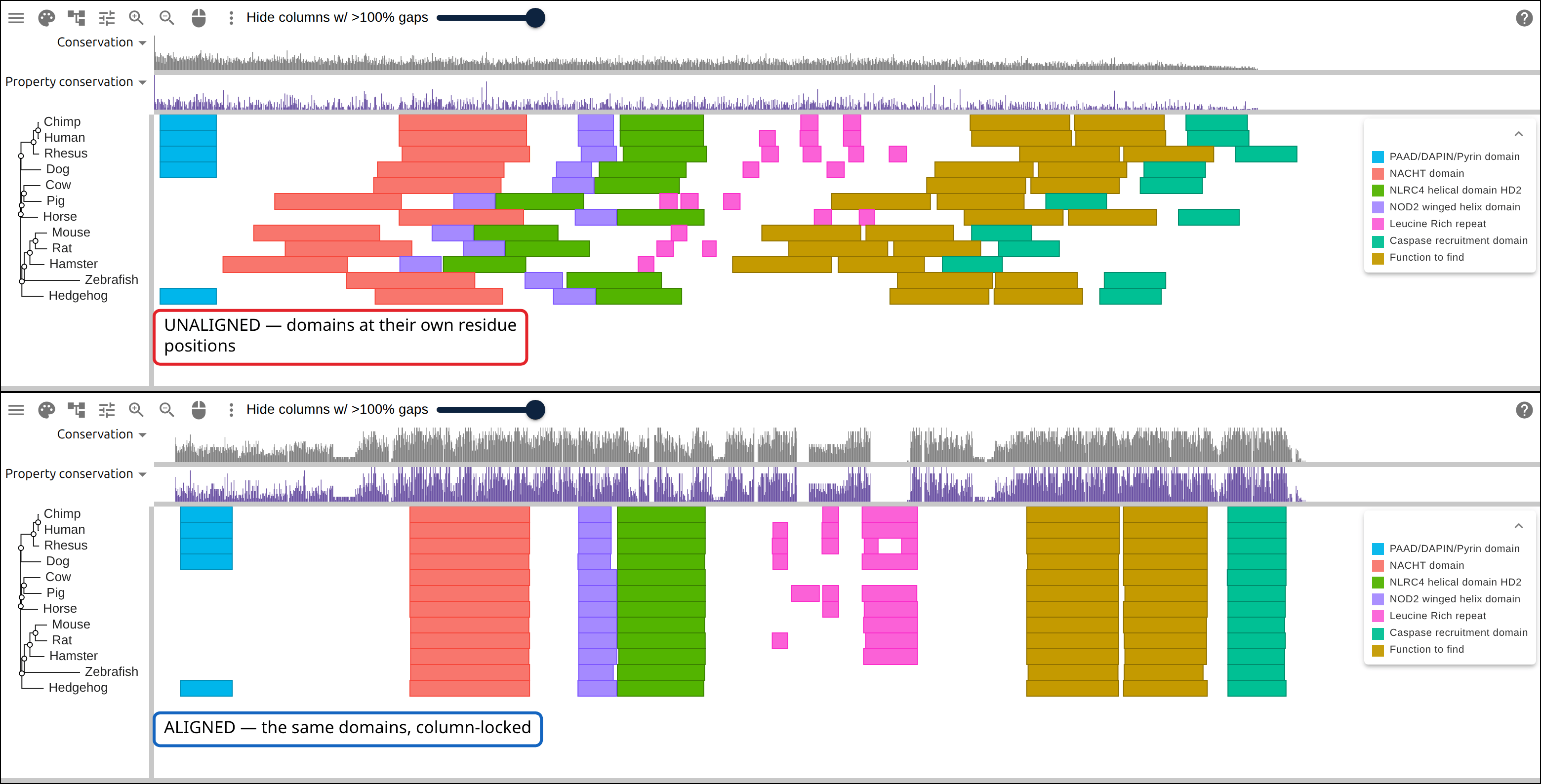
Load a GFF3 annotation file from the import form, or from Annotations → Open annotation file…, to overlay domains on the alignment. The overlay accepts any GFF3, including exon and gene models; InterProScan output is the most common input. The dialog also takes the JSON an InterProScan run returns and converts it to GFF3 as it loads. Either way the annotations travel in the shared link with the rest of the view. The viewer translates each row’s annotation coordinates into alignment columns, so they line up across the family even where gaps shift the underlying sequence positions.
The CLI builds the file:
react-msaview-cli interpro reads InterPro’s precomputed matches for UniProt
accessions in seconds, and interproscan scans sequences InterPro has not seen.
The
protein family tutorial
walks through both, and Annotations → How to get a domain file… opens it
from the app.
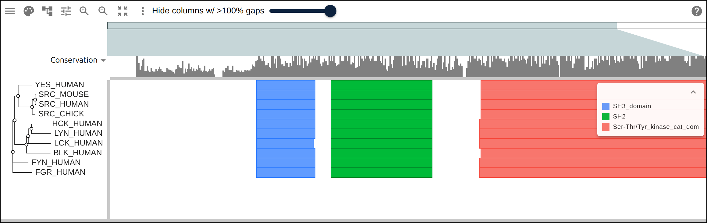
react-msaview-cli interproscan. Zoomed out to full length, the shared SH3,
SH2, and tyrosine-kinase catalytic domain architecture lines up across every
member.Why the overlay is column-locked#
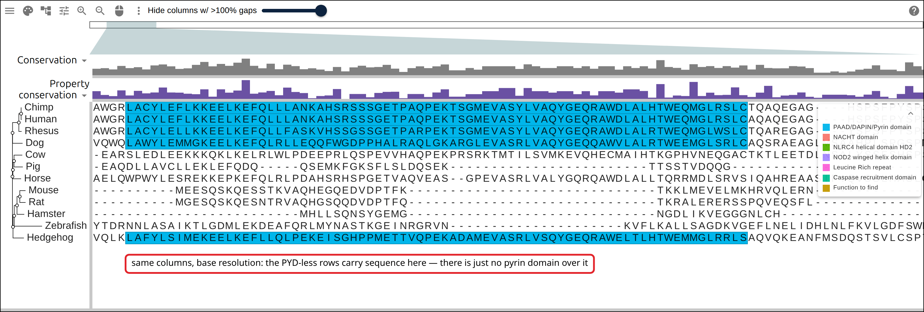
The two panels below show what the translation into alignment columns changes. Both hold the same twelve NLRP1 orthologs, domain GFF, component, palette and tree; only the bottom panel’s input was aligned.
Viewing metadata#
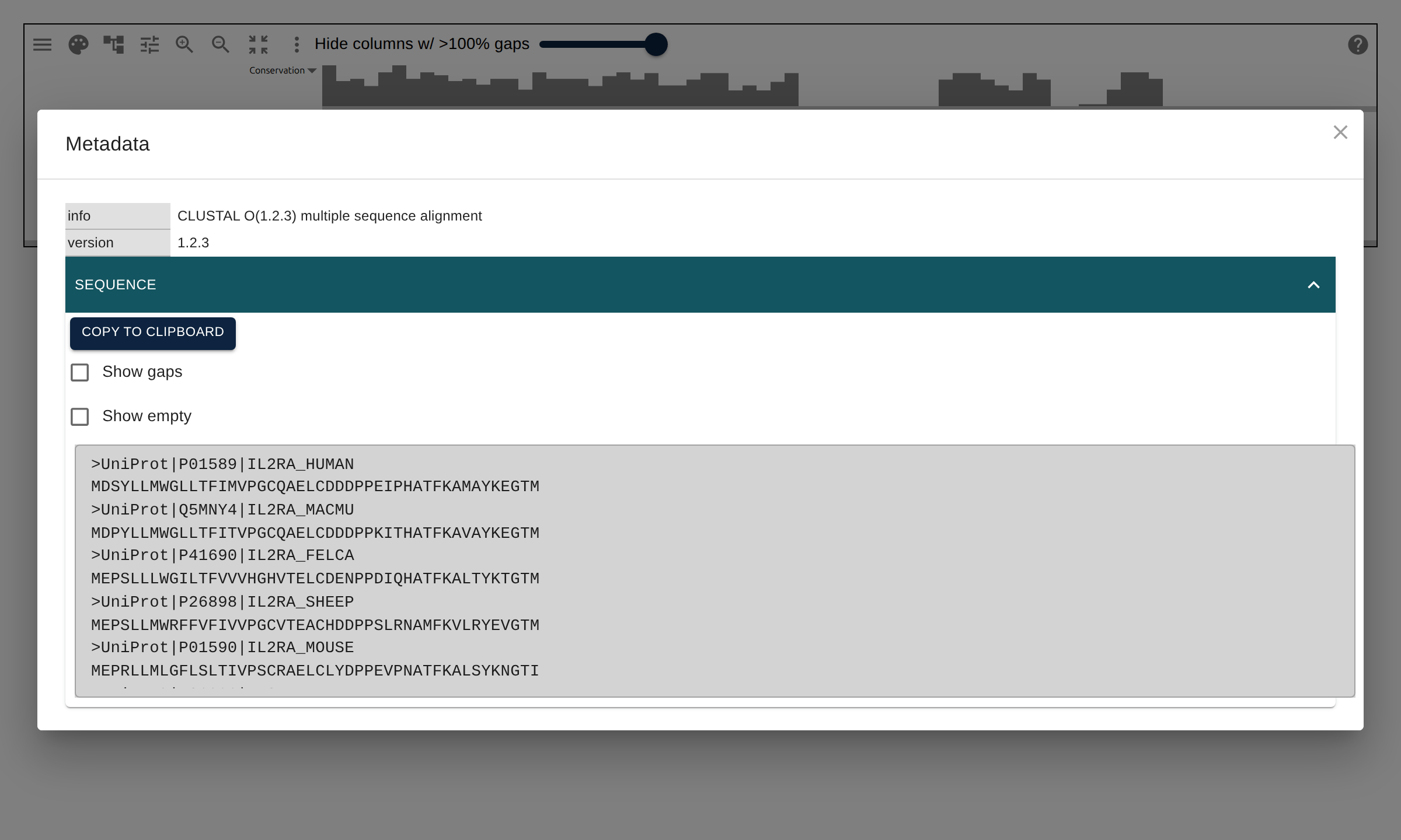
Alignment file headers and per-sequence information are available from the Metadata dialog (file menu).
Sharing and exporting#
- Share a session with Copy link above the viewer, which copies the page URL as of the click. The URL encodes the view state (colors, zoom, collapsed clades, highlights), so a collaborator who opens the link sees the same view. A file you opened from your own computer goes into the link too, up to a size limit described under Link to a view.
- Point at something before you share. The snapshot carries labeled highlights: a residue of a named sequence, a column range, or a set of rows, each with a note drawn beside it. The view state stores them (see the layers reference), so a link can open on a band labeled “R248, conserved in 651 of 658 orthologs”.
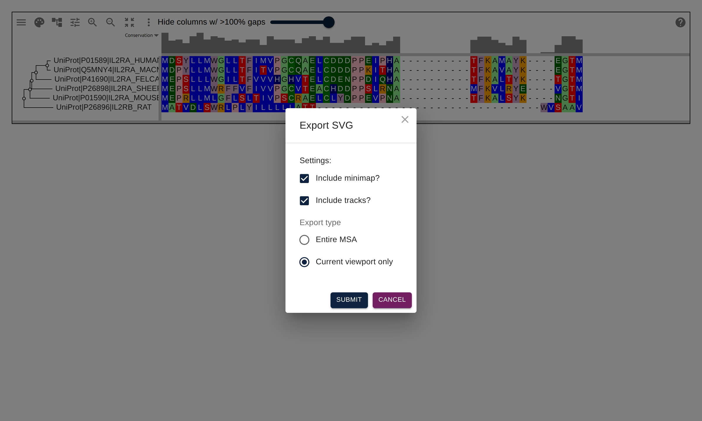
- Export an image with Export SVG (file menu): a vector figure of the current viewport or the entire alignment, optionally with the minimap and annotation tracks.
Link to a view#
Besides Copy link, a script can build a link. The app reads the view from
the URL’s fragment, #data=, holding the URL-encoded JSON of the view. A link
written with the ?data= query parameter, as older links were, opens too, and
the app moves it into the fragment.
const view = {
  type: 'MsaView',
  msaFilehandle: { uri: 'https://example.org/kinase.aln' },
  colorSchemeName: 'clustalx_protein_dynamic',
  highlights: [{ row: 'SRC_HUMAN', start: 530, end: 530, label: 'Y530' }],
}
const url = `https://gmod.org/JBrowseMSA/demo/#data=${encodeURIComponent(JSON.stringify(view))}`
Either that bare MsaView snapshot or the {"msaview": {...}} wrapper the app
writes back to the address bar works. The
layers reference and the
model API docs
list every field. When the app cannot read a snapshot, it opens on an error
naming the problem, not on the import form.
Three things decide whether the link works for the person who opens it:
- Where the files live. The app resolves a
uriagainst its own address, sodata/kinase.alnmeansgmod.org/JBrowseMSA/demo/data/kinase.aln. That works for the hosted examples and fails for a link you send, so use an absolute URL. - CORS. The browser fetches those URLs from
gmod.org, so the server holding them has to sendAccess-Control-Allow-Origin. GitHub Pages, S3 with a CORS rule, and the public EBI/NCBI/PDBe APIs send it. Most institutional web servers and Google Drive do not, and the view then opens on a fetch error. - Size. The browser never sends a URL’s fragment to the server, so the
length of a
#data=link is up to the browser: Chrome and Firefox both open one of 1,000,000 characters. The app gzips the snapshot and inlines a pasted or locally opened file up to 1 MB; a 400 kB protein alignment encodes to about 305,000 characters. A larger file stays in the running viewer but leaves the snapshot, and the header shows Not in the link. When a file is too large, or the whole view still encodes past 1,000,000 characters, the app removes#data=so the address bar never holds a URL that opens empty, and Copy link turns off and says why. To share a larger file, serve it over HTTP and open it by URL; the link then stores the address, which works at any file size. The same 1 MB limit applies to a data track.
Tracks#
Tracks are strips drawn above the alignment, sharing its columns and its horizontal scroll. The Tracks submenu at the top of the MSA settings menu lists every track and turns each on or off. The dropdown arrow on a track’s label, at the left, also closes it and shows its details.
Hovering a track reads out what it draws at that column: the two conservation scores, the sequence logo’s information content and residue composition, the columns an arc joins, the letter on a text track. Show track values on hover in the MSA settings menu turns the readout off. Over the alignment itself, the tooltip carries the domains and insertions under the cursor, and the header reads out the hovered row, residue and position.
- Conservation: a per-column histogram of how conserved the column is, from Shannon entropy, scaled down by the column’s gap fraction. On by default.
- Property conservation: the same measure over physicochemical property class instead of exact identity. It shows sites held constant by conservative substitution, which identity-based conservation counts as variable. Protein alignments only, on by default.
- Sequence logo: the residues of each column stacked by the information they carry, tallest on top, each letter’s height its share of the column’s total. Off by default. Column height is information content in bits, so it tops out at log2(20) for protein and log2(4) for nucleotide, and a column whose residues are evenly split draws nothing at all. Frequencies come from the non-gap residues, and the track then scales the whole stack by the column’s occupancy, so a column that is mostly gaps stays short even when its few residues agree.
- Position: column numbers with a tick under each, at whatever spacing the zoom leaves room for. Off by default. The track counts alignment columns. When the view is drawn relative to a row (Indicate differences from this row in a row’s menu), it counts that row’s residues and skips the columns where the row has a gap.
- Secondary structure and the other annotation rows a Stockholm file carries
inline appear as text tracks, colored by the active scheme. Every
#=GCline gets one:SS_cons,seq_cons, Rfam’sRFand motif lines. Every#=GRline gets one too, named<row> <tag>, but starts hidden, since a Pfam seed carries a couple of per-row active-site lines and an Rfam family carries a structure line per row with a PDB entry. Turn them on from Settings → Tracks. - Base pairs: the same
#=GC SS_consannotation drawn as arcs joining the columns that pair, shown whenever a Stockholm file carries one. Pseudoknot pairs get their own color. WUSS writes those pairs asA/abecause they cross a helix and brackets can only nest; the arcs show the crossing.
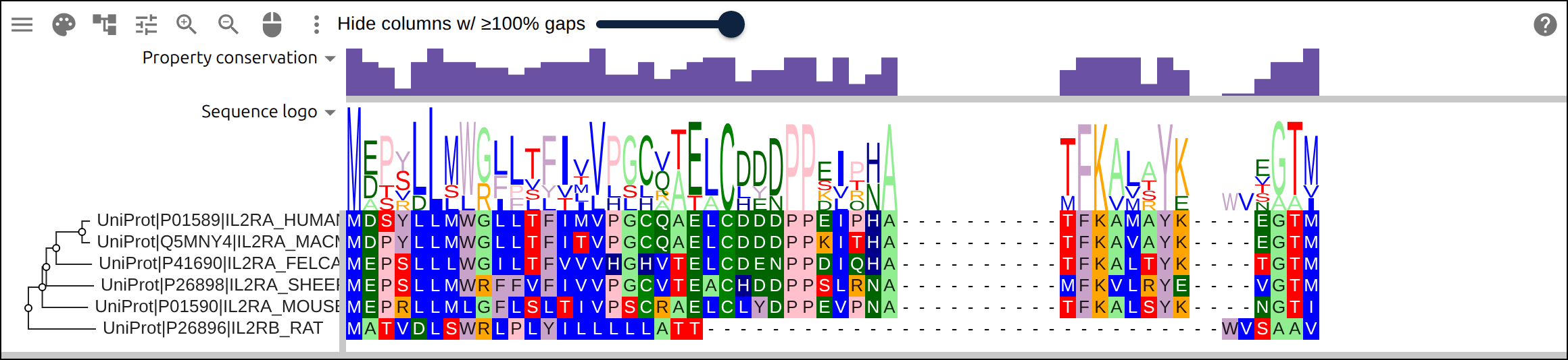
- in the rows
below it.Check “Include tracks?” in the export dialog to include tracks in an SVG export.
A host can also supply a track as data. A columnTracks entry in the shared URL
or session carries per-column values drawn as bars, a per-column string drawn
like a Stockholm annotation line, or pairs of positions drawn as arcs. Values
can index alignment columns or the residues of one row, and each track gets a
name, a color and its own menu entry. Use an arc track for a pairing: a
disulfide bond, a residue contact from a structure, a base pair the file does
not already annotate. The layers reference
lists the fields.
Settings reference#
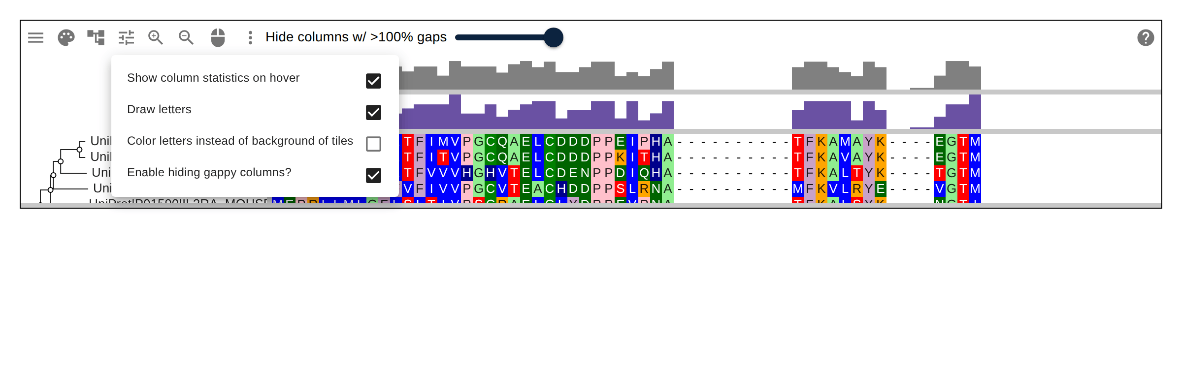
Layout options live in two dropdowns in the header: MSA settings and tree settings, beside the color-scheme palette.
Scaling to large data#
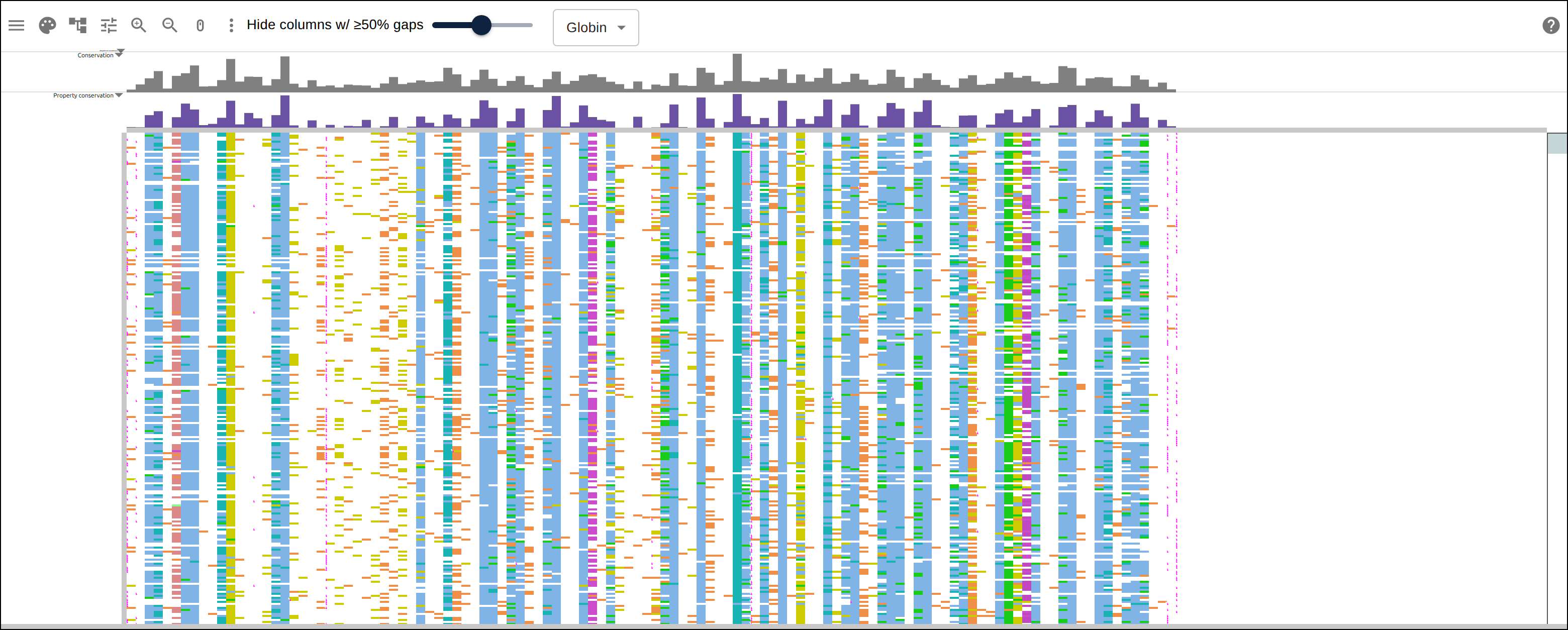
The viewer tiles both axes, so memory and draw time grow with the visible area, not with the size of the file.
Embedding and related projects#
- Embedding guide: React, UMD-in-HTML, and the R package.
- JBrowse 2 integration: the viewer as a view inside JBrowse 2, connected to a genome view and 3D structure.
- jbrowse-plugin-msaview: the JBrowse 2 plugin (demo).
- ProteinBrowser: a protein-analysis suite built on this viewer.