Influenza drift in a notebook
The H3N2 vaccine is reformulated because the virus’s hemagglutinin changes where
antibodies bind it. This page takes the 25 H3N2 strains chosen for the northern
hemisphere vaccine between 1968 and 2022, aligns their hemagglutinin, counts how
often each column changed from one strain to the next, and draws the result in
Jupyter with msaview-widget. The alignment carries its own control: the HA2
fusion peptide, which has to stay the same for the protein to work, sits in the
same 567 columns as the antigenic sites that change every few years.
Prerequisites#
- Python 3.10 or newer, in a notebook (JupyterLab, Jupyter Notebook, VS Code, Colab, or marimo)
pip install msaview-widget biopython numpy pandas- ClustalW,
apt install clustalwon Debian or Ubuntu,brew install clustal-won macOS
Every figure below links to the live view it captured.
Where the data comes from#
NCBI protein records, one per vaccine strain, fetched by accession so a rerun aligns the same sequences.
- the records, in one request: https://eutils.ncbi.nlm.nih.gov/entrez/eutils/efetch.fcgi?db=protein&id=AFG71887.1,YGK08660.1&rettype=fasta&retmode=text
- the strains, as WHO published them: https://www.who.int/teams/global-influenza-programme/vaccines/who-recommendations
- the alignment the commands below write, hosted so the figures can link to it: https://gmod.org/JBrowseMSA/demo/data/h3n2/h3n2-ha.aln
- its tree: https://gmod.org/JBrowseMSA/demo/data/h3n2/h3n2-ha.nh
- the layers the notebook computed: https://gmod.org/JBrowseMSA/demo/data/h3n2/h3n2-layers.json
1. The strains#
Each row is a year, the strain WHO named for that season, and the accession of a full-length HA0 record for it.
STRAINS = [
    (1968, "A/Hong Kong/1/1968", "AFG71887.1"),
    (1972, "A/England/42/1972", "AFM71912.1"),
    (1975, "A/Victoria/3/1975", "AFG98995.1"),
    # ... 21 more, through
    (2021, "A/Darwin/9/2021", "XZO11388.1"),
    (2022, "A/Massachusetts/18/2022", "YGK08660.1"),
]

strains = pd.DataFrame(STRAINS, columns=["year", "strain", "accession"])
strains["row"] = [
    f"{year}_{strain.split('/')[1].replace(' ', '')}"
    for year, strain in zip(strains.year, strains.strain)
]
Each accession came from one Entrez search of the protein database for the
strain name, "A/Darwin/9/2021"[All Fields] AND hemagglutinin[Protein Name]. A
strain has several records, some of them partial, and the one kept is the
full-length HA0 of 566 residues. The build script at the bottom of this page
pins the list above, because a search run next year can return a different first
hit.
strains.row is the label the viewer draws down the side: the year first, so
the rows sort by date and a Newick tip name carries no space.
2. Fetch the records#
with Entrez.efetch(
    db="protein", id=",".join(strains.accession), rettype="fasta", retmode="text"
) as handle:
    records = {r.id: r for r in SeqIO.parse(handle, "fasta")}

for row, accession in zip(strains.row, strains.accession):
    records[accession].id = row
    records[accession].description = ""

ordered = [records[a] for a in strains.accession]
SeqIO.write(ordered, "h3n2-ha.fasta", "fasta")
year strain accession length
1968 A/Hong Kong/1/1968 AFG71887.1 566
1972 A/England/42/1972 AFM71912.1 566
1975 A/Victoria/3/1975 AFG98995.1 566
... ... ... ...
2021 A/Darwin/9/2021 XZO11388.1 566
2022 A/Massachusetts/18/2022 YGK08660.1 566All 25 are 566 residues: a 16-residue signal peptide, then HA1 at 329 residues, then HA2. H3 numbering counts from HA1’s first residue, so every position quoted below is that number plus 16.
3. Align#
subprocess.run(
    ["clustalw", "-INFILE=h3n2-ha.fasta", "-ALIGN", "-TYPE=PROTEIN",
     "-OUTPUT=FASTA", "-OUTFILE=h3n2-ha.aln"],
    check=True,
)
aligned = {r.id: r for r in SeqIO.parse("h3n2-ha.aln", "fasta")}
SeqIO.write([aligned[row] for row in strains.row], "h3n2-ha.aln", "fasta")
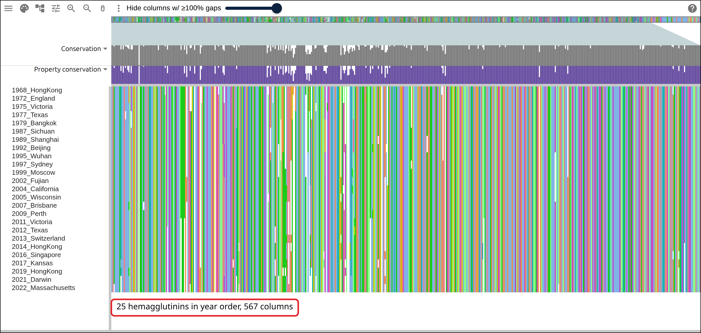
alignment: 25 rows x 567 columnsThe second write puts the rows back in year order. ClustalW writes its output in guide-tree order, and the viewer draws the rows in the order the file gives them, so without the rewrite the first row is a 2013 strain.
4. A tree, and a date check#
Biopython builds the distance matrix and the neighbor-joining tree, and the tree carries no year.
msa = MultipleSeqAlignment([aligned[row] for row in strains.row])
tree = DistanceTreeConstructor().nj(DistanceCalculator("blosum62").get_distance(msa))
tree.root_with_outgroup(strains.row[0])
Phylo.write(tree, "h3n2-ha.nh", "newick")
A tree built from sequences alone can be checked against the dates the sequences came with. Distance from the 1968 root should grow with the year:
depth = tree.depths()
distance = [depth[t] for t in tree.get_terminals()]
year = [int(t.name.split("_")[0]) for t in tree.get_terminals()]
np.corrcoef(distance, year)[0, 1]
root-to-tip distance against year: r = 0.985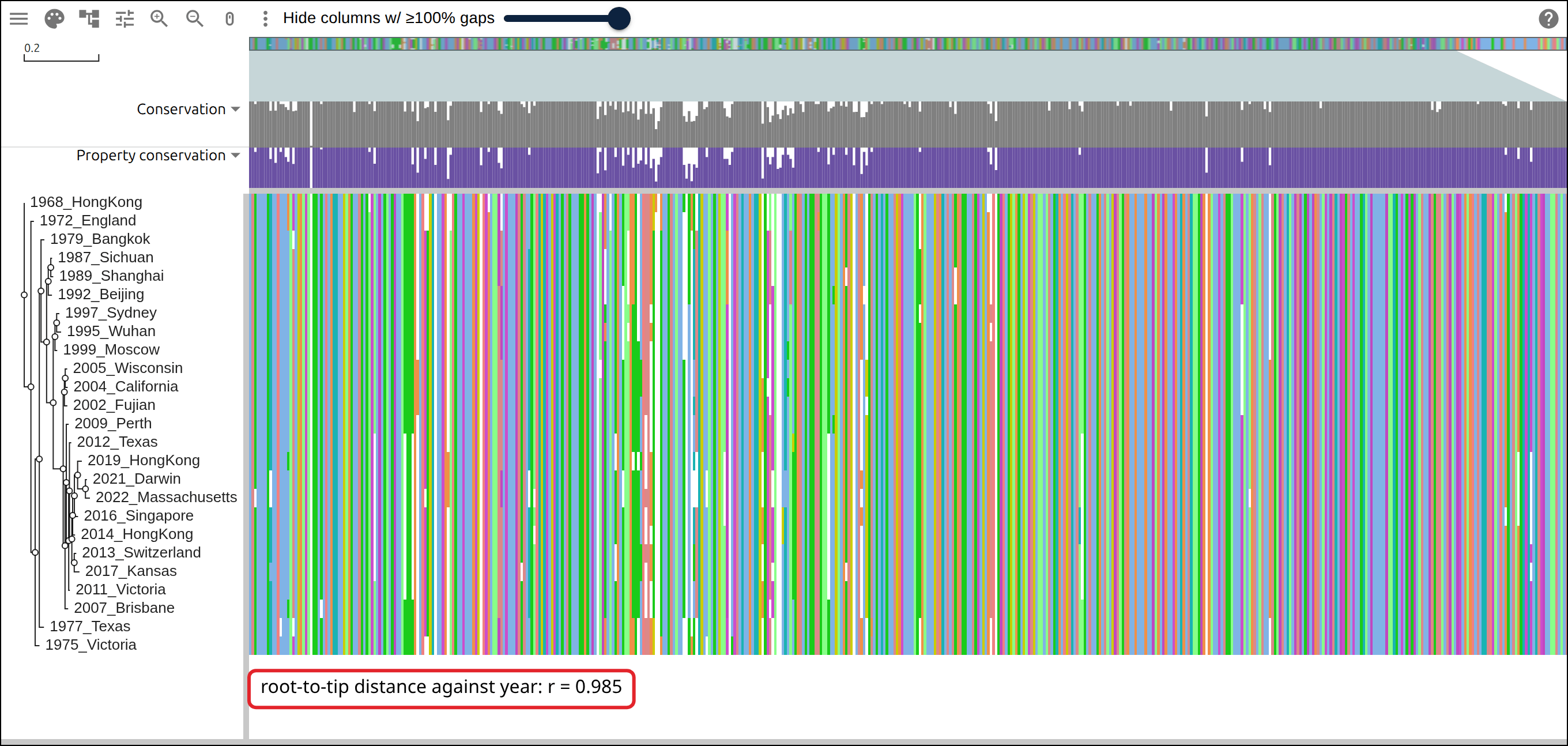
5. Count the changes the alignment carries#
The viewer’s conservation track reads a column across all 25 rows at once. A series that runs in time supports a different count: how often the letter changed from one vaccine strain to the next.
columns = np.array([list(str(aligned[row].seq)) for row in strains.row])
changes = (columns[:-1] != columns[1:]).sum(axis=0)
columns that never changed: 449 of 567
the busiest column changed 11 times
the 2022 strain matches the 1968 one in 479 of 567 columnsFour fifths of the columns hold the same letter from one strain to the next all
the way through, and the 2022 strain matches the 1968 one in 479 of the 567. The
column_tracks trait takes the counts as one bar per column:
drift = {
    "id": "drift",
    "name": "Changes between consecutive strains",
    "kind": "bar",
    "values": changes,
    "max": int(changes.max()),
    "color": "#c0392b",
    "height": 60,
}
values takes a numpy array as it is.
6. Mark the antigenic sites and the fusion peptide#
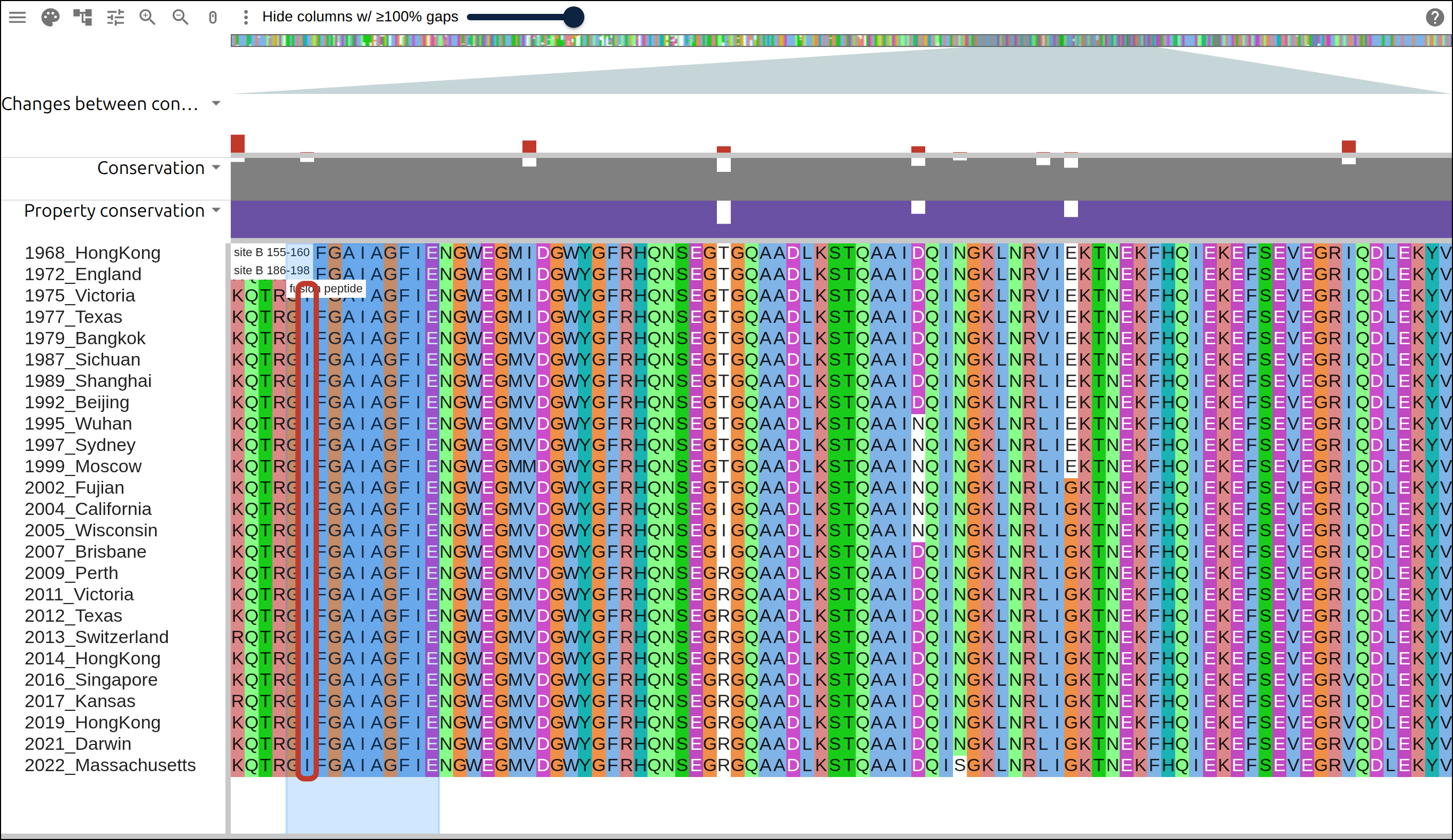
Antigenic site B is two stretches of HA1, 155 to 160 and 186 to 198, on the rim of the receptor-binding site. The fusion peptide is the first 11 residues of HA2, which insert into the endosome membrane. Both go in as highlights on the 1968 row, and the viewer projects a row’s residues onto columns:
SIGNAL, HA1_LENGTH = 16, 329
reference = strains.row[0]

def h3(position):
    """H3 numbering -> residue of the record, which counts the signal peptide."""
    return position + SIGNAL

bands = [
    {"row": reference, "start": h3(155), "end": h3(160), "label": "site B 155-160"},
    {"row": reference, "start": h3(186), "end": h3(198), "label": "site B 186-198"},
    {"row": reference, "start": h3(HA1_LENGTH + 1), "end": h3(HA1_LENGTH + 11),
     "label": "fusion peptide", "color": "rgba(0,120,255,0.18)"},
]
Everything so far goes into the widget in one call:
from msaview import MSAView

view = MSAView(
    msa="h3n2-ha.aln",
    tree="h3n2-ha.nh",
    column_tracks=[drift],
    highlights=bands,
    relative_to=reference,
    col_width=2.2,
    row_height=16,
    height=700,
)
view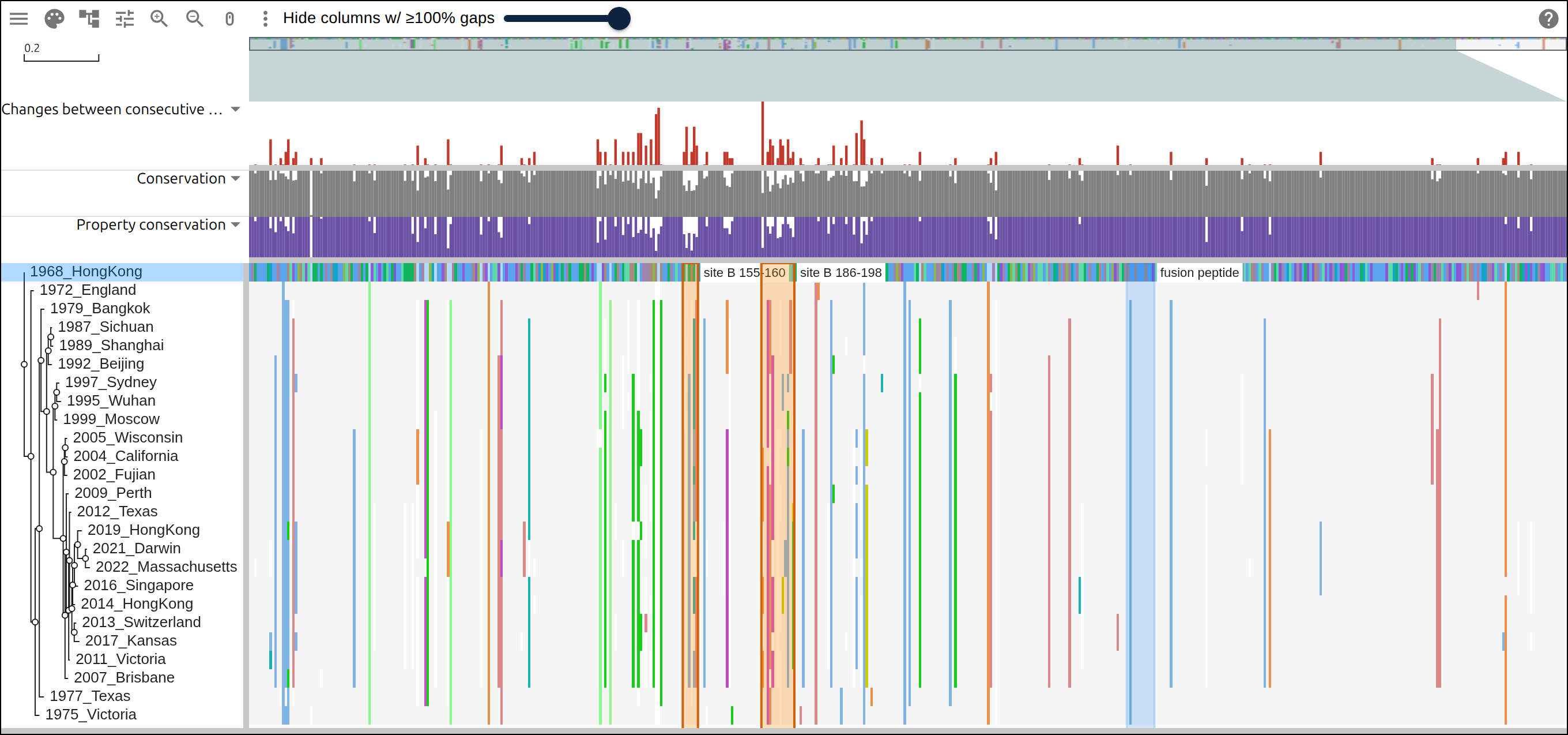
relative_to drawing every row as its
differences from 1968. The two orange bands are site B, the blue band is the
fusion peptide, and the red bars stand highest in HA1.7. Read the two regions#
residue_column = np.cumsum([c != "-" for c in str(aligned[reference].seq)])

def column_of(residue):
    return int(np.argmax(residue_column == residue))

site_b = [h3(p) for start, end in [(155, 160), (186, 198)] for p in range(start, end + 1)]
fusion = list(range(h3(HA1_LENGTH + 1), h3(HA1_LENGTH + 11) + 1))
def read(positions):
    at = [column_of(r) for r in positions]
    return ["".join(columns[i, at]) for i in range(len(strains))]

pd.DataFrame({
    "year": strains.year,
    "site B (155-160, 186-198)": read(site_b),
    "fusion peptide (HA2 1-11)": read(fusion),
})
year site B (155-160, 186-198) fusion peptide (HA2 1-11)
1968 TKSGSTSTNQEQTSLYVQA GLFGAIAGFIE
1972 YKSGSTSTNQEQTSLYVQA GLFGAIAGFIE
1975 YKSGSTSTDKEQTDLYVQA GIFGAIAGFIE
1977 YKSESTSTDKEQTNLYVQA GIFGAIAGFIE
1979 YESESKSTDKEQTNLYVRA GIFGAIAGFIE
1987 YKSEYKVTDREQTNLYVRA GIFGAIAGFIE
1989 HESEYKITDREQTNLYVRA GIFGAIAGFIE
1992 HKSEYKSTDRDQTSLYVRA GIFGAIAGFIE
1995 HKLEYKSTDSDQTSIYVQA GIFGAIAGFIE
1997 HQLKYKSTDSDQTSIYAQA GIFGAIAGFIE
1999 HQLKYRSTDSDQTSLYTQA GIFGAIAGFIE
2002 THLKYKGTDSDQISLYAQA GIFGAIAGFIE
2004 THLKFKGTNNDQISLYTQA GIFGAIAGFIE
2005 THLKFKVTDNDQIFLYAQA GIFGAIAGFIE
2007 THLKFKGTDNDQIFLYAQA GIFGAIAGFIE
2009 THLNFKGTDKDQIFLYAQA GIFGAIAGFIE
2011 THLNFKGTDKDQIFLYAQS GIFGAIAGFIE
2012 THLNFKGTDKDQIFLYAQP GIFGAIAGFIE
2013 THLNSKVTDKDQIFLYAQS GIFGAIAGFIE
2014 THLNYKGTDKDQIFPYAQS GIFGAIAGFIE
2016 THLNYKGTDKDQIFPYAQS GIFGAIAGFIE
2017 THLNSKVTDKNQISLYAQS GIFGAIAGFIE
2019 THLNYIVTDKDQISLYAQS GIFGAIAGFIE
2021 TSLNNINTDKNQISLFAQS GIFGAIAGFIE
2022 TSLNNIDTDKNQFSLFAQS GIFGAIAGFIEsite B reads 24 distinct strings in 25 strains, the fusion peptide 2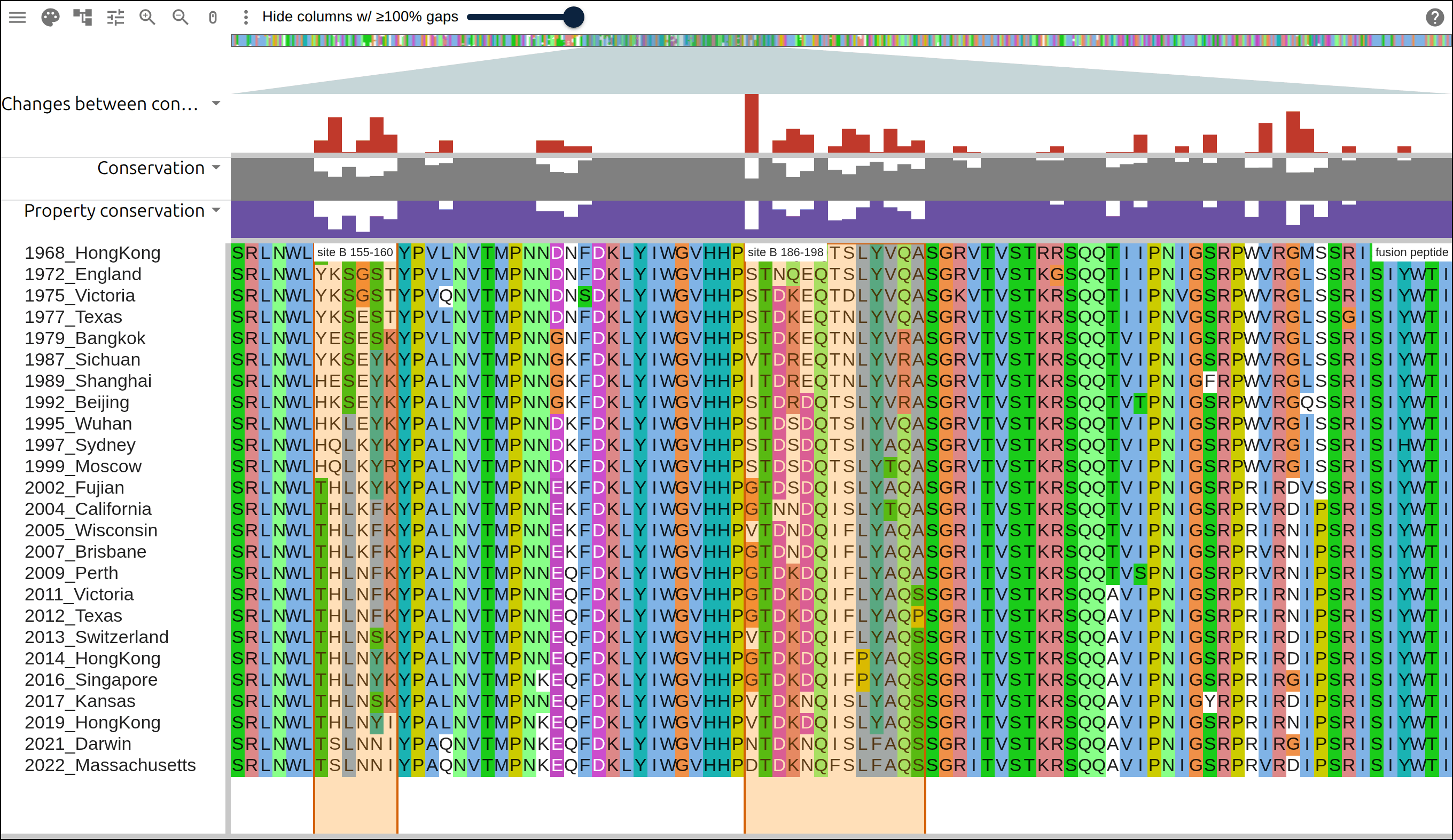
8. The loop back to Python#
The widget sets two traits from the browser. clicked holds the cell a click
pinned, and viewport holds the columns on screen:
def show(change):
    cell = change["new"]
    if cell:
        print(cell["row"], cell["column"], cell["letter"])

view.observe(show, "clicked")
Both are 1-based, column counts every column of the alignment, and residue
counts the clicked row’s own letters. A click on a column of the figure above
answers with the year, the column and the residue, which indexes straight back
into the DataFrame:
view.observe(
    lambda change: display(
        pd.DataFrame({
            "year": strains.year,
            "letter": columns[:, change["new"]["column"] - 1],
        })
    ),
    "clicked",
)
Setting a trait redraws the widget in place and keeps its scroll and zoom, so a
cell that changes view.color_scheme or view.highlights restyles the view
above it.
9. Share the link#
The same layers go into a URL that opens the hosted alignment in the web viewer, for a reader with no kernel:
snapshot = {"msaview": {
    "type": "MsaView",
    "height": 560,
    "colWidth": 2.2,
    "rowHeight": 16,
    "colorSchemeName": "clustalx_protein_dynamic",
    "msaFilehandle": {"uri": "data/h3n2/h3n2-ha.aln"},
    "treeFilehandle": {"uri": "data/h3n2/h3n2-ha.nh"},
    "columnTracks": [{**drift, "values": changes.tolist()}],
    "highlights": bands,
}}
"https://gmod.org/JBrowseMSA/demo/#data=" + urllib.parse.quote(
    json.dumps(snapshot, separators=(",", ":")), safe=""
)
the link is 3332 charactersjson.dumps needs changes.tolist(), where the widget took the numpy array
whole.
Reproduce it end to end#
curl -O https://raw.githubusercontent.com/GMOD/JBrowseMSA/main/docs/tutorials/scripts/build_flu_drift.py
python build_flu_drift.py out/
The script runs every command above and writes out/h3n2-ha.aln,
out/h3n2-ha.nh and out/h3n2-layers.json, the files the links on this page
open. The numbers quoted here are the ones it prints.
See also#
- Python package, with the example notebooks and every trait
- Data layers
- A protease family in R
- JBrowse 2 integration, which opens an alignment beside a genome and a structure
References#
- Wiley DC, Wilson IA, Skehel JJ. Structural identification of the antibody-binding sites of Hong Kong influenza haemagglutinin and their involvement in antigenic variation. Nature 289:373-378 (1981), which named sites A through E.
- Skehel JJ, Wiley DC. Receptor binding and membrane fusion in virus entry: the influenza hemagglutinin. Annual Review of Biochemistry 69:531-569 (2000).
- Smith DJ, et al. Mapping the antigenic and genetic evolution of influenza virus. Science 305:371-376 (2004).
- Koel BF, et al. Substitutions near the receptor binding site determine major antigenic change during influenza virus evolution. Science 342:976-979 (2013).
- Cock PJA, et al. Biopython: freely available Python tools for computational molecular biology and bioinformatics. Bioinformatics 25:1422-1423 (2009).
- Larkin MA, et al. Clustal W and Clustal X version 2.0. Bioinformatics 23:2947-2948 (2007).