Hemoglobin’s two subunits and the interfaces between them
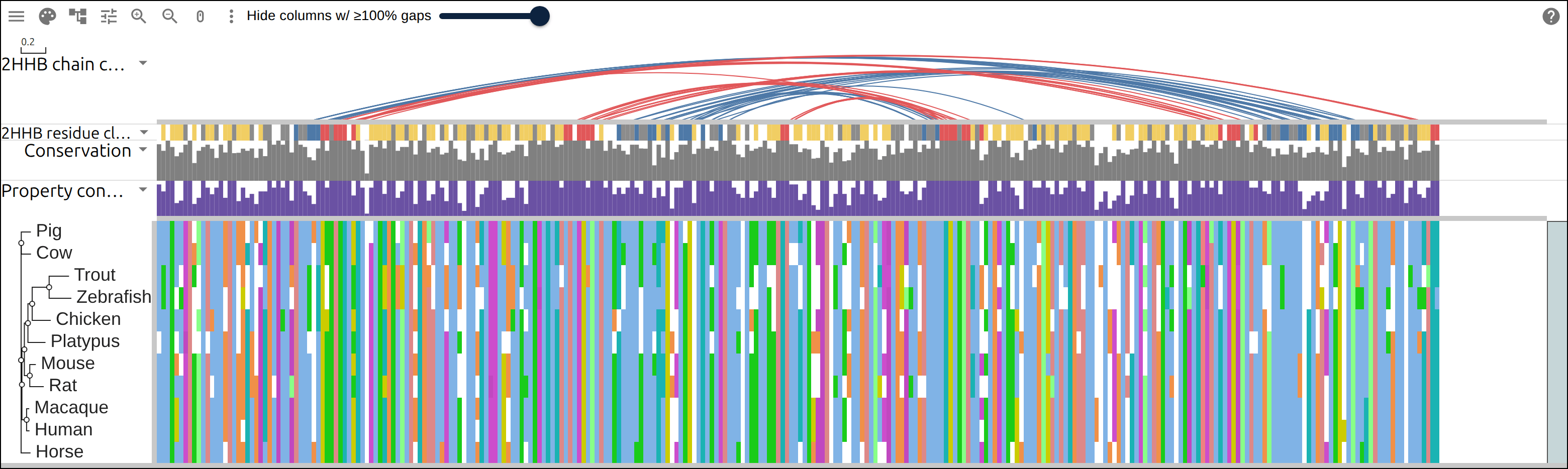
Hemoglobin is a tetramer of two alpha and two beta chains, and the residues that hold it together sit on two kinds of interface: alpha1beta1, the packing contacts that keep a dimer together, and alpha1beta2, the sliding contacts that move when the tetramer binds oxygen. The viewer holds one sequence per row, so this page gives each species one row with its alpha and its beta concatenated, and draws every residue pair in contact between two chains of PDB 2HHB as an arc from the alpha block to the beta block. Eleven vertebrates, 22 RefSeq proteins, and the last section reads how conserved each interface is against the residues on the surface, which touch nothing.
Prerequisites#
curl- ClustalW,
apt install clustalwon Debian or Ubuntu,brew install clustal-won macOS. ClustalW both aligns and infers a tree, so this page needs no other aligner. - python3 with Biopython,
pip install biopython, for the contacts and the solvent exposure
Every figure below links to the live view it captured.
Where the data comes from#
Twenty-two globin proteins as NCBI RefSeq holds them, and one crystal structure from RCSB.
- all 22 protein sequences, one request: https://eutils.ncbi.nlm.nih.gov/entrez/eutils/efetch.fcgi?db=protein&id=NP_000549.1,NP_000509.1&rettype=fasta&retmode=text
- the human deoxyhemoglobin tetramer, PDB 2HHB, as mmCIF: https://files.rcsb.org/download/2HHB.cif
- the row table the commands below start from, hosted so the figures can link to it: https://gmod.org/JBrowseMSA/demo/data/hemoglobin/hemoglobin-rows.tsv
- the alignment they write: https://gmod.org/JBrowseMSA/demo/data/hemoglobin/hemoglobin.afa
- its tree: https://gmod.org/JBrowseMSA/demo/data/hemoglobin/hemoglobin.nwk
- the subunit spans: https://gmod.org/JBrowseMSA/demo/data/hemoglobin/hemoglobin-subunits.gff
- the contacts and the chain mappings, the layers the links below carry: https://gmod.org/JBrowseMSA/demo/data/hemoglobin/hemoglobin-layers.json
1. Name the rows#
Write one species per line: the label the viewer draws, then the RefSeq protein
for the alpha subunit and for the beta subunit. The label becomes the FASTA
defline, the tree tip, the GFF seq_id and the row of every layer.
Human	NP_000549.1	NP_000509.1
Macaque	NP_001038189.1	NP_001157900.1
Mouse	NP_032244.2	NP_001188320.1
Rat	NP_001007723.1	NP_942071.2
Cow	NP_001070890.2	NP_776342.1
Pig	NP_001432111.1	NP_001138313.1
Horse	NP_001078901.1	NP_001157490.1
Platypus	XP_028905054.1	XP_028913684.1
Chicken	NP_001004376.1	NP_990820.1
Zebrafish	NP_571332.3	NP_001003431.2
Trout	NP_001118023.1	XP_021413554.1
Seven placental mammals, a monotreme, a bird and two fish. The human pair is HBA1 and HBB; each other species contributes its adult alpha and adult beta chain.
2. Fetch the sequences#
One efetch request takes every accession, and a short script splits the result
into one FASTA per subunit, with the species label as the defline so the two
files pair up by name:
ids=$(awk -F'\t' '{printf "%s%s,%s", sep, $2, $3; sep=","}' rows.tsv)
curl -sf "https://eutils.ncbi.nlm.nih.gov/entrez/eutils/efetch.fcgi?db=protein&id=$ids&rettype=fasta&retmode=text" \
  -o globins-ncbi.fasta
Human alpha NP_000549.1 142 aa beta NP_000509.1 147 aa
Macaque alpha NP_001038189.1 142 aa beta NP_001157900.1 147 aa
Mouse alpha NP_032244.2 142 aa beta NP_001188320.1 147 aa
Rat alpha NP_001007723.1 142 aa beta NP_942071.2 147 aa
Cow alpha NP_001070890.2 142 aa beta NP_776342.1 145 aa
Pig alpha NP_001432111.1 142 aa beta NP_001138313.1 147 aa
Horse alpha NP_001078901.1 142 aa beta NP_001157490.1 147 aa
Platypus alpha XP_028905054.1 141 aa beta XP_028913684.1 147 aa
Chicken alpha NP_001004376.1 142 aa beta NP_990820.1 147 aa
Zebrafish alpha NP_571332.3 143 aa beta NP_001003431.2 147 aa
Trout alpha NP_001118023.1 143 aa beta XP_021413554.1 147 aaEvery alpha is 141 to 143 residues and every beta 145 to 147, initiator methionine included. The Cow beta is two residues short at the N terminus, and the two fish alphas carry one extra.
3. Align each subunit on its own#
Alpha and beta are paralogs, and an aligner given both would put them in shared columns. Each subunit gets its own alignment, and the two are joined per species afterwards:
for sub in alpha beta; do
  clustalw -INFILE=$sub.fasta -ALIGN -TYPE=PROTEIN -OUTORDER=INPUT \
    -OUTPUT=FASTA -OUTFILE=$sub.afa
done
-OUTORDER=INPUT keeps the rows in the table’s order, so the two files line up
by position as well as by name. Concatenating them is a loop over the labels:
alpha = read('alpha.afa')
beta = read('beta.afa')
with open('hemoglobin.afa', 'w') as fh:
    for name, a in alpha.items():
        fh.write(f'>{name}\n{a}{beta[name]}\n')
alpha: 143 columns, beta: 147 columns
concatenated: 290 columns, beta starts at column 144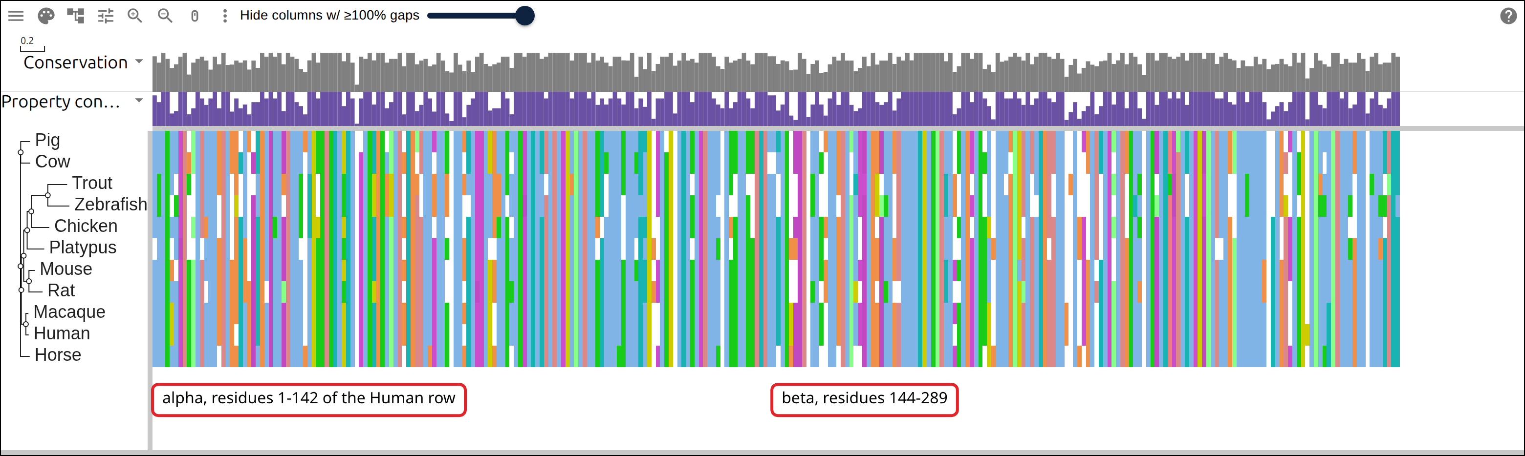
4. Mark the subunits#
A GFF gives every row its two spans, in that row’s own residue numbering, so the
boundary lands on the right residue in the rows whose alpha is one residue
shorter or longer. A color= attribute on each line sets the overlay’s color:
alen = len(a.replace('-', ''))
blen = len(b.replace('-', ''))
g.write(f'{name}\tRefSeq\tpolypeptide_region\t1\t{alen}\t.\t.\t.\t'
        f'Name=alpha;signature_desc=hemoglobin subunit alpha;color=%234e79a7\n')
g.write(f'{name}\tRefSeq\tpolypeptide_region\t{alen + 1}\t{alen + blen}\t.\t.\t.\t'
        f'Name=beta;signature_desc=hemoglobin subunit beta;color=%23e15759\n')
Human RefSeq polypeptide_region 1 142 . . . Name=alpha;signature_desc=hemoglobin subunit alpha;color=%234e79a7
Human RefSeq polypeptide_region 143 289 . . . Name=beta;signature_desc=hemoglobin subunit beta;color=%23e15759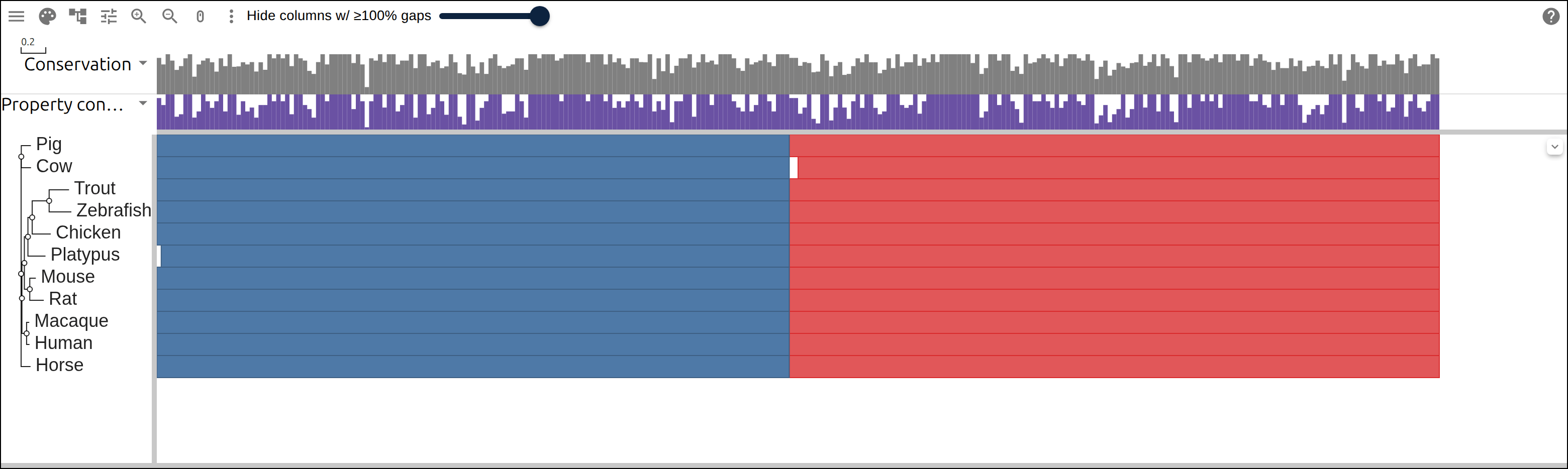
5. Infer a tree#
clustalw -INFILE=hemoglobin.afa -TREE -TYPE=PROTEIN -OUTPUTTREE=phylip
tr -d '[:space:]' < hemoglobin.ph > hemoglobin.nwk
(((Human:0.02366,Macaque:0.02133):0.03786,((Mouse:0.04913,Rat:0.11350):0.04393,
(Platypus:0.14248,(Chicken:0.15042,(Zebrafish:0.18011,Trout:0.16126):0.13737):0.03453)
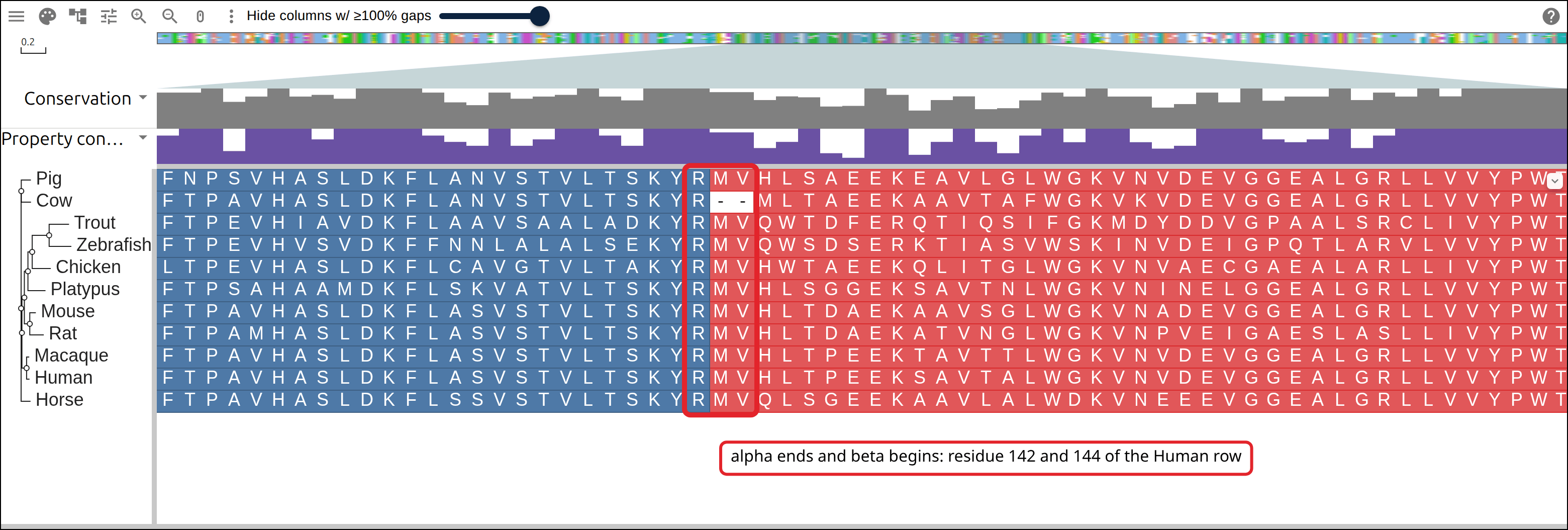
:0.02900):0.01972):0.00663,(Cow:0.07886,Pig:0.07794):0.00138,Horse:0.07648);The two fish sit together at the end of the longest branch, Chicken joins them next, then Platypus, and the seven placentals fill the rest of the tree.
6. Read the contacts off the structure#
2HHB is the human deoxy tetramer at 1.74 Å. Chains A and C are alpha, B and D
are beta; chain A touches B across the alpha1beta1 interface and D across
alpha1beta2. Biopython’s NeighborSearch finds every residue pair with a heavy
atom of each within 4 Å:
from Bio.PDB import MMCIFParser, NeighborSearch

def contacts(c1, c2, cutoff=4.0):
    ns = NeighborSearch([a for r in c2 for a in r])
    pairs = set()
    for r in c1:
        for atom in r:
            for other in ns.search(atom.coord, cutoff):
                pairs.add((r.id[1], other.get_parent().id[1]))
    return sorted(pairs)

model = MMCIFParser(QUIET=True).get_structure('2HHB', '2hhb.cif')[0]
alpha1beta1 = contacts(model['A'], model['B'])
alpha1beta2 = contacts(model['A'], model['D'])
The RefSeq rows keep the initiator methionine and the mature chains in the crystal do not, so the script finds each chain’s sequence inside the Human row before trusting a single number:
chain A (141 aa) is row residues 2-142 of Human, chain B (146 aa) is 144-289
the Human row is 289 residues: alpha 1-142, beta 143-289
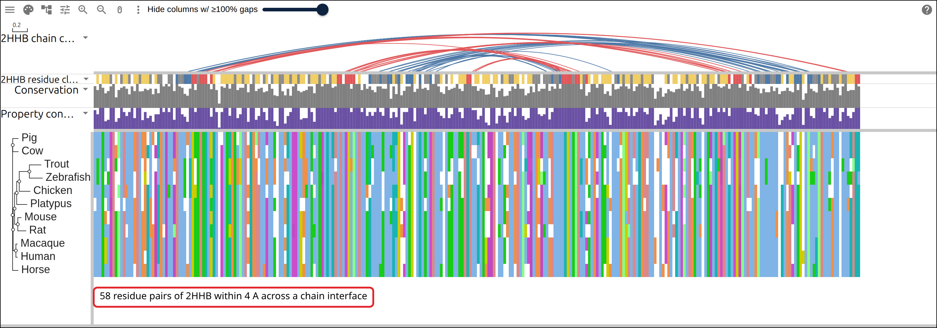
alpha1beta1: 32 residue pairs within 4.0 A, 14 alpha residues and 17 beta residues
alpha1beta2: 26 residue pairs within 4.0 A, 14 alpha residues and 14 beta residues
Chain residue n is row residue n + 1 within its subunit, and beta residue n is
row residue 143 + n. Every pair becomes an arc from its alpha column to its beta
column, colored by interface, in an arc column track over the Human row. A
second, text track gives every residue of that row a class: 1 and 2 for
the two interfaces, and for the rest, B where the residue is buried in the
assembled tetramer, E where it is exposed, and O between. The exposure comes
from Biopython’s ShrakeRupley over the whole tetramer, divided by the residue
type’s maximum accessible area:
residue classes on the Human row: 29 at alpha1beta1, 28 at alpha1beta2, 73 buried, 107 exposed, 52 in betweenThe script also writes two residueMappings records for the Human row, one per
chain, so a host can look any residue of the row up in the structure.
7. How conserved each class is#
For every residue of the Human row, the share of the ten other rows carrying the same letter in that column, averaged per class:
alpha1beta1 interface     29 residues, mean identity 0.77, 10 identical in all 11 rows
alpha1beta2 interface     28 residues, mean identity 0.92, 20 identical in all 11 rows
buried, no interface      73 residues, mean identity 0.78, 21 identical in all 11 rows
exposed, no interface    107 residues, mean identity 0.69, 22 identical in all 11 rows
23 of 58 contact pairs have both residues identical in all 11 rows
The alpha1beta2 residues are the most conserved class in the row: 20 of the 28 are identical from human to trout, and the mean identity is above the buried core’s. The alpha1beta1 residues match the core, and the exposed residues, which touch no other chain, are the lowest of the four.
8. Check it against the raw data#
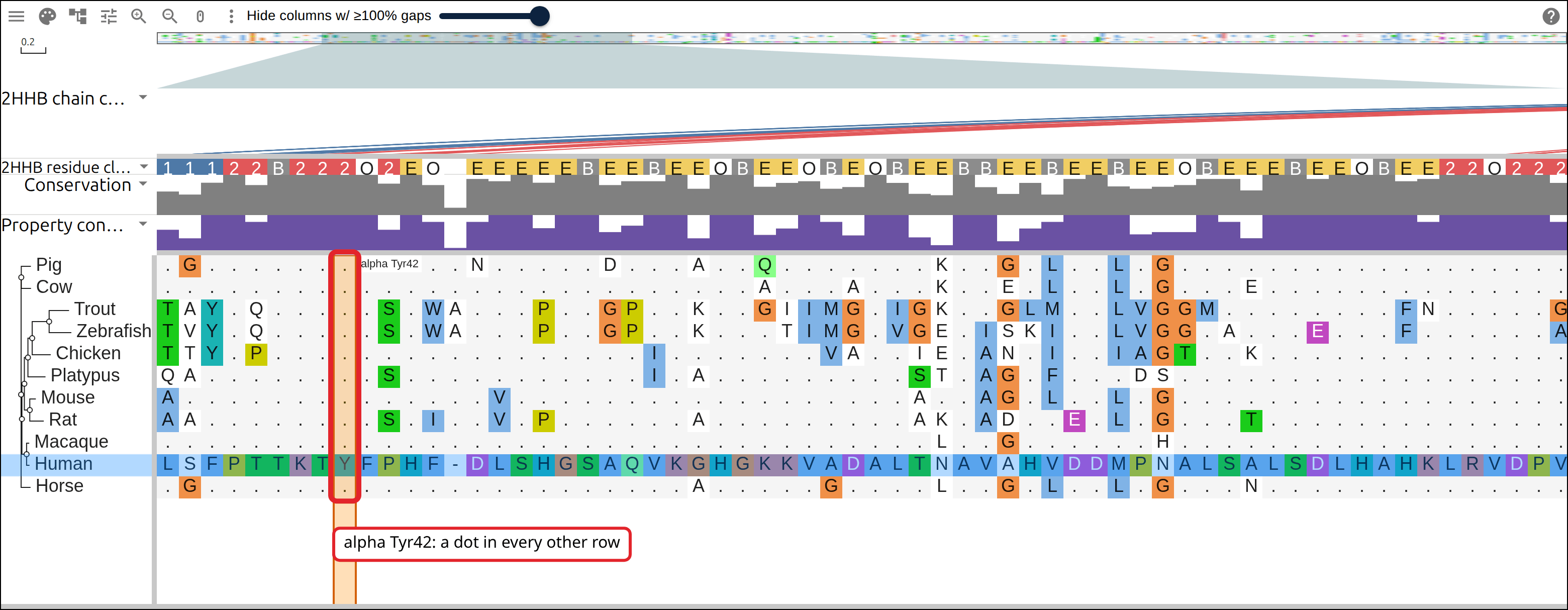
The script prints the letters every row carries at one pair per interface, the Tyr42 to Asp99 pair and the alpha1beta1 pair that varies most:
alpha1beta2 Tyr42-Asp99: row residues 43 and 242, columns 43 and 243
  Human      Y D
  Macaque    Y D
  Mouse      Y D
  Rat        Y D
  Cow        Y D
  Pig        Y D
  Horse      Y D
  Platypus   Y D
  Chicken    Y D
  Zebrafish  Y D
  Trout      Y D
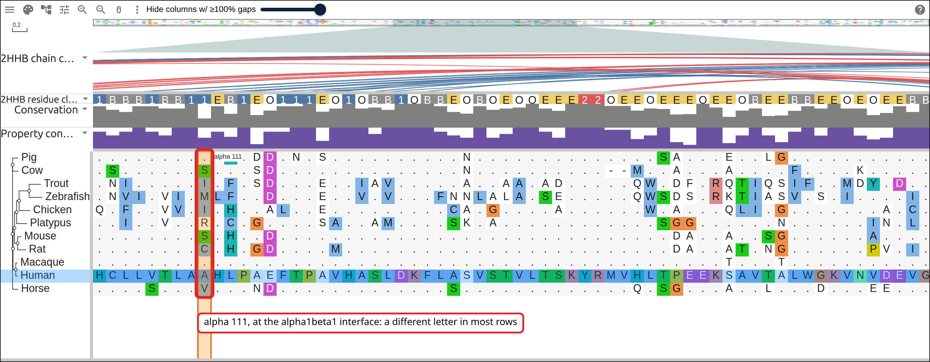
alpha1beta1, most variable: row residues 112 and 258, columns 113 and 259
  Human      A A
  Macaque    A A
  Mouse      S G
  Rat        C G
  Cow        S A
  Pig        A A
  Horse      V A
  Platypus   R A
  Chicken    I A
  Zebrafish  M A
  Trout      I A
Alpha 111 and beta 115 pack against each other in the crystal, and across the eleven rows the alpha side reads seven different letters.
9. Open the whole thing#
The view combines three hosted files and three layers. The files go behind URLs, and the layers go in the link, because they take a few kilobytes:
{
  "msaview": {
    "type": "MsaView",
    "colWidth": 4.4,
    "rowHeight": 22,
    "colorSchemeName": "clustalx_protein_dynamic",
    "msaFilehandle": { "uri": "https://example.org/hemoglobin.afa" },
    "treeFilehandle": { "uri": "https://example.org/hemoglobin.nwk" },
    "gffFilehandle": { "uri": "https://example.org/hemoglobin-subunits.gff" },
    "showDomains": false
  }
}
Add the columnTracks and residueMappings entries from
hemoglobin-layers.json beside those, URL-encode the whole object, and hang it
off the app as #data=.
A host that loads this view can look a residue of the Human row up in either chain. The two mappings share an entry id, so the reverse lookup needs the chain:
model.structureResidue('Human', 43) // 2HHB chain A, residue 42
model.structureResidue('Human', 242) // 2HHB chain B, residue 99
model.structureResidue('Human', 143) // undefined: the beta initiator, in no chain
model.rowResidue('2HHB', 42) // undefined: both chains have a residue 42
model.rowResidue('2HHB', 42, 'A') // Human, residue 43
Reproduce it end to end#
curl -O https://raw.githubusercontent.com/GMOD/JBrowseMSA/main/docs/tutorials/scripts/build_protein_complex.sh
bash build_protein_complex.sh
With no arguments the script writes the row table above and builds all four files beside it, printing every number on this page. Pass your own table to do the same for another complex and another structure:
bash build_protein_complex.sh my-rows.tsv out/See also#
- Data layers
- The SARS-CoV-2 furin insert and PDB 6VXX
- An alignment linked to its structure
- A protein family from a list of accessions
- User guide
References#
- Fermi G, Perutz MF, Shaanan B, Fourme R. The crystal structure of human deoxyhaemoglobin at 1.74 Å resolution. J Mol Biol 175:159-174.
- Perutz MF. Stereochemistry of cooperative effects in haemoglobin. Nature 228:726-739.
- Baldwin J, Chothia C. Haemoglobin: the structural changes related to ligand binding and its allosteric mechanism. J Mol Biol 129:175-220.
- Tien MZ, Meyer AG, Sydykova DK, Spielman SJ, Wilke CO. Maximum allowed solvent accessibilites of residues in proteins. PLoS ONE 8:e80635.
- Cock PJA, Antao T, Chang JT, et al. Biopython: freely available Python tools for computational molecular biology and bioinformatics. Bioinformatics 25:1422-1423.