An RSV phylogeny from a public Nextstrain build
A phylogenetic tree with a dozen tips fits on a screen with room to read every label. A public health lab tracking a virus works with a tree two orders of magnitude bigger: one tip per genome sequenced that season, thousands of them, related by descent within one species. This page takes one such tree, a public Nextstrain build of respiratory syncytial virus, reconstructs an alignment and tree from it that an alignment viewer can open, and shows how collapsing, subsampling and zooming make 1,840 rows readable.
Prerequisites#
curl- Python 3, standard library only, nothing to install
- nothing to read along: every figure below links to the live view it captured
Where the data comes from#
Nextstrain’s RSV-A build, updated 2024-07-16: a tree over 1,840 genomes, one ancestral sequence, and the nucleotide substitutions on every branch between them.
- the auspice JSON itself: https://data.nextstrain.org/rsv_a_genome.json
- the full-tip alignment the build script reconstructs from it, sliced to the G gene, hosted so the figures can link to it: https://gmod.org/JBrowseMSA/demo/data/scale/rsv-full.aln
- its tree: https://gmod.org/JBrowseMSA/demo/data/scale/rsv-full.nh
- the subsampled whole-genome alignment the later figures use: https://gmod.org/JBrowseMSA/demo/data/scale/rsv-sample.aln
- its tree: https://gmod.org/JBrowseMSA/demo/data/scale/rsv-sample.nh
The genome#
RSV-A’s genome is 15,225 nucleotides, eleven genes from NS1 to L. Two of them anchor this page. G, the attachment glycoprotein, carries the ectodomain that takes the brunt of antibody selection. L, the polymerase, replicates the genome and tolerates change in almost none of its residues. Nextstrain’s pipeline places every sampled genome in a tree but publishes no alignment of them, so the first step builds one.
1. Reconstruct the alignment from the tree#
Every branch in the JSON carries the nucleotide substitutions that happened on it, numbered against one embedded reference sequence. Copying that reference down each root-to-tip path, overwriting one base per mutation as you go, produces every tip’s full genome in the same 15,225 coordinates the reference uses:
def reconstruct(node, seq):
    for m in node["branch_attrs"]["mutations"].get("nuc", []):
        pos, alt = int(m[1:-1]), m[-1]
        seq = seq[: pos - 1] + alt + seq[pos:]
    if not node.get("children"):
        tips.append((node["name"], seq))
    else:
        for child in node["children"]:
            reconstruct(child, seq)
reconstructed 1840 tip sequences, genome length 15225
G gene 4652-5617 (966 nt)
L gene 8532-15029 (6498 nt)The rows come out already aligned: a substitution changes a base without moving anything around it, and this dataset carries no insertion relative to the reference. A deletion becomes a run of gap characters at a fixed position, which fits an alignment column.
2. The whole tree at once#
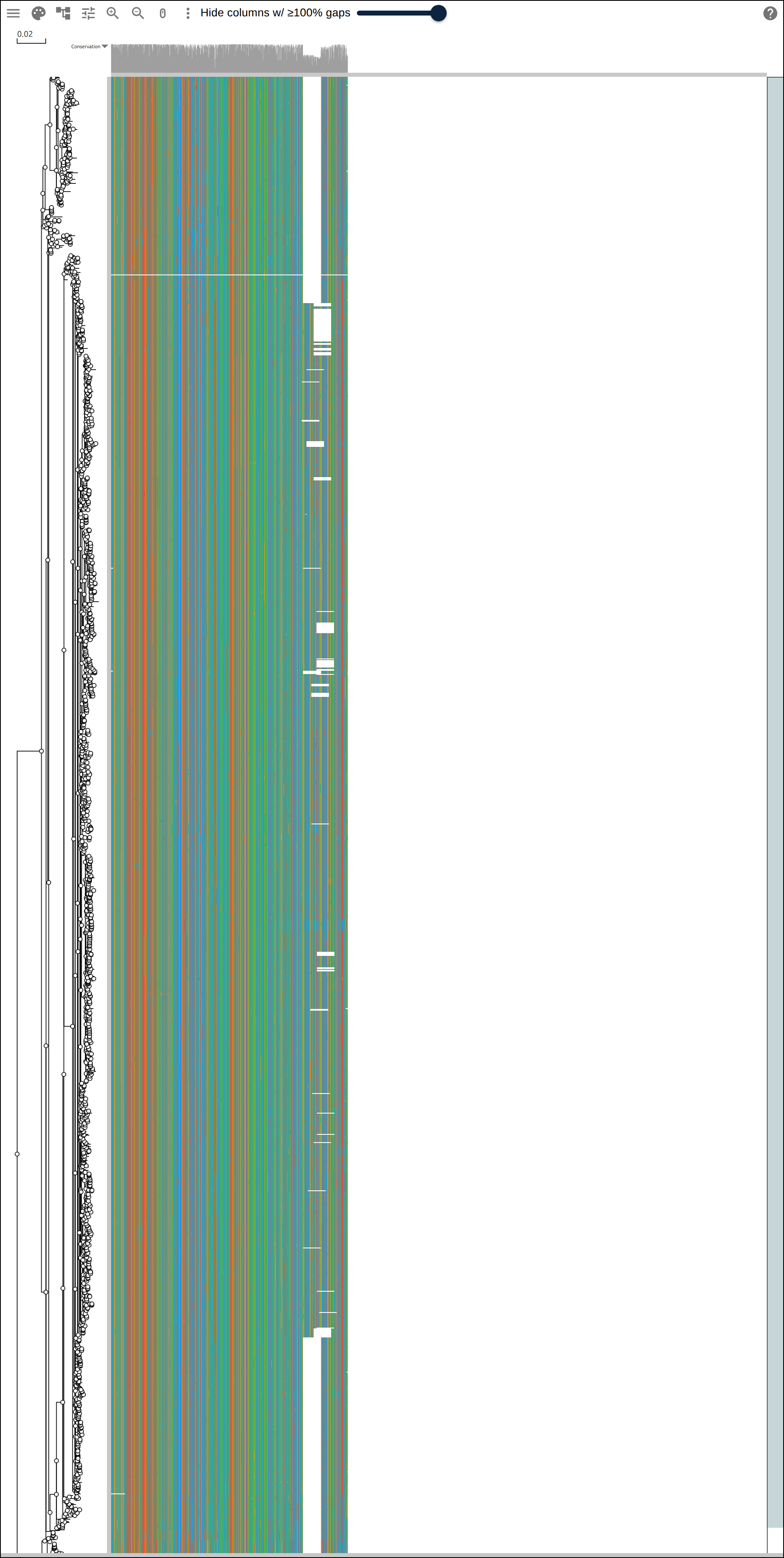
The first view draws all 1,840 tips at one pixel of row height, next to the alignment sliced to the G gene.
3. Collapse a clade#
Clicking a node in the tree collapses everything under it into one triangle. The build script picks a clade whose descendants all share one clade call and one country:
collapse target: node-0-0-1, 49 tips, clade A.1, all USA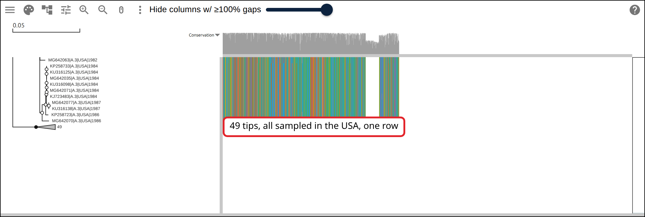
4. Subsample for a readable page#
Row labels and letters are not readable at 1,840 rows, so the remaining figures use every 10th tip in the file’s order. The selection is deterministic, so a reader reproducing it on their own tree needs no random seed.
subsample: 184 of 1840 tips (every 10th)
23 of 24 clades represented in the subsample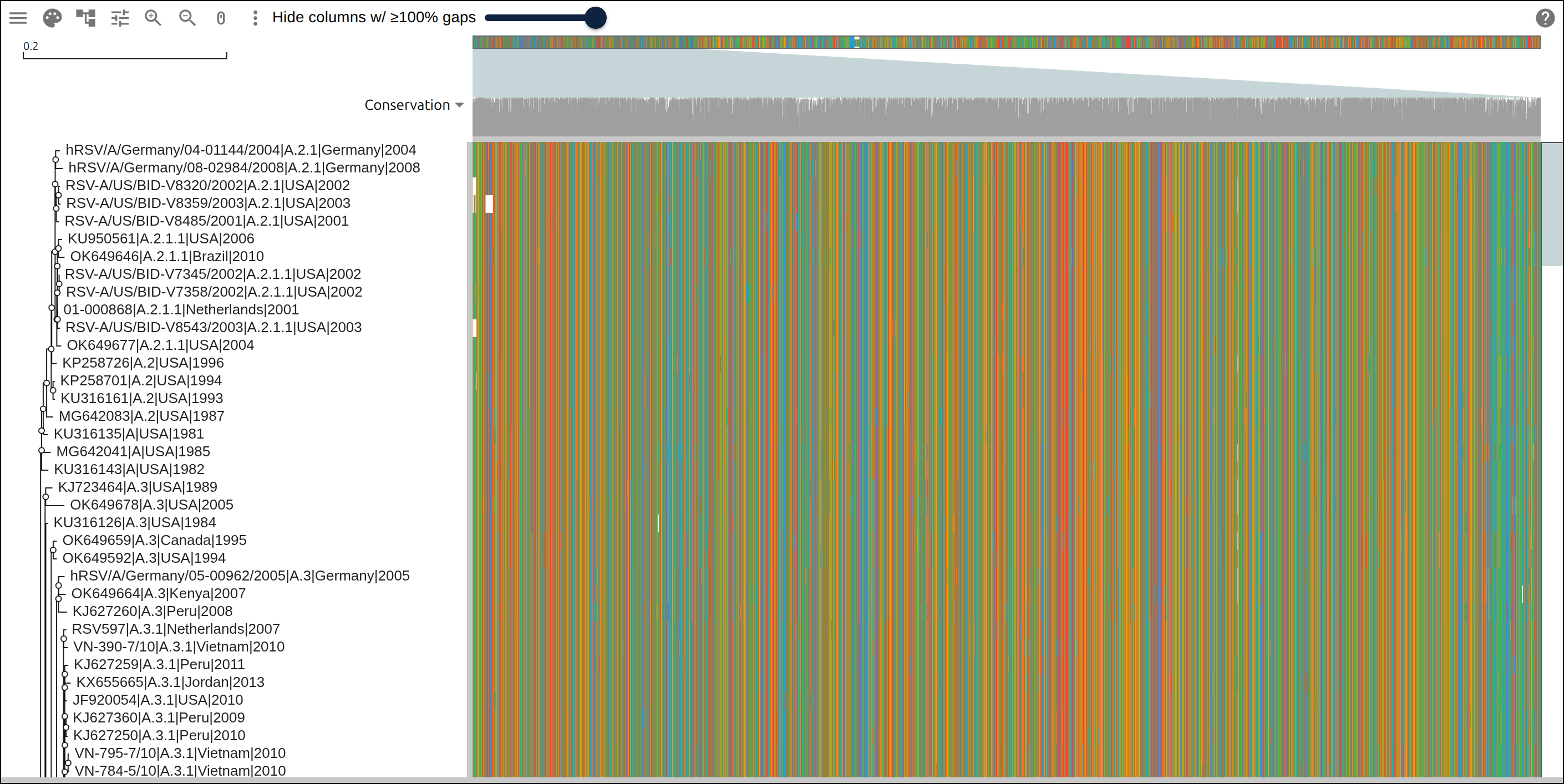
5. Group rows by clade#
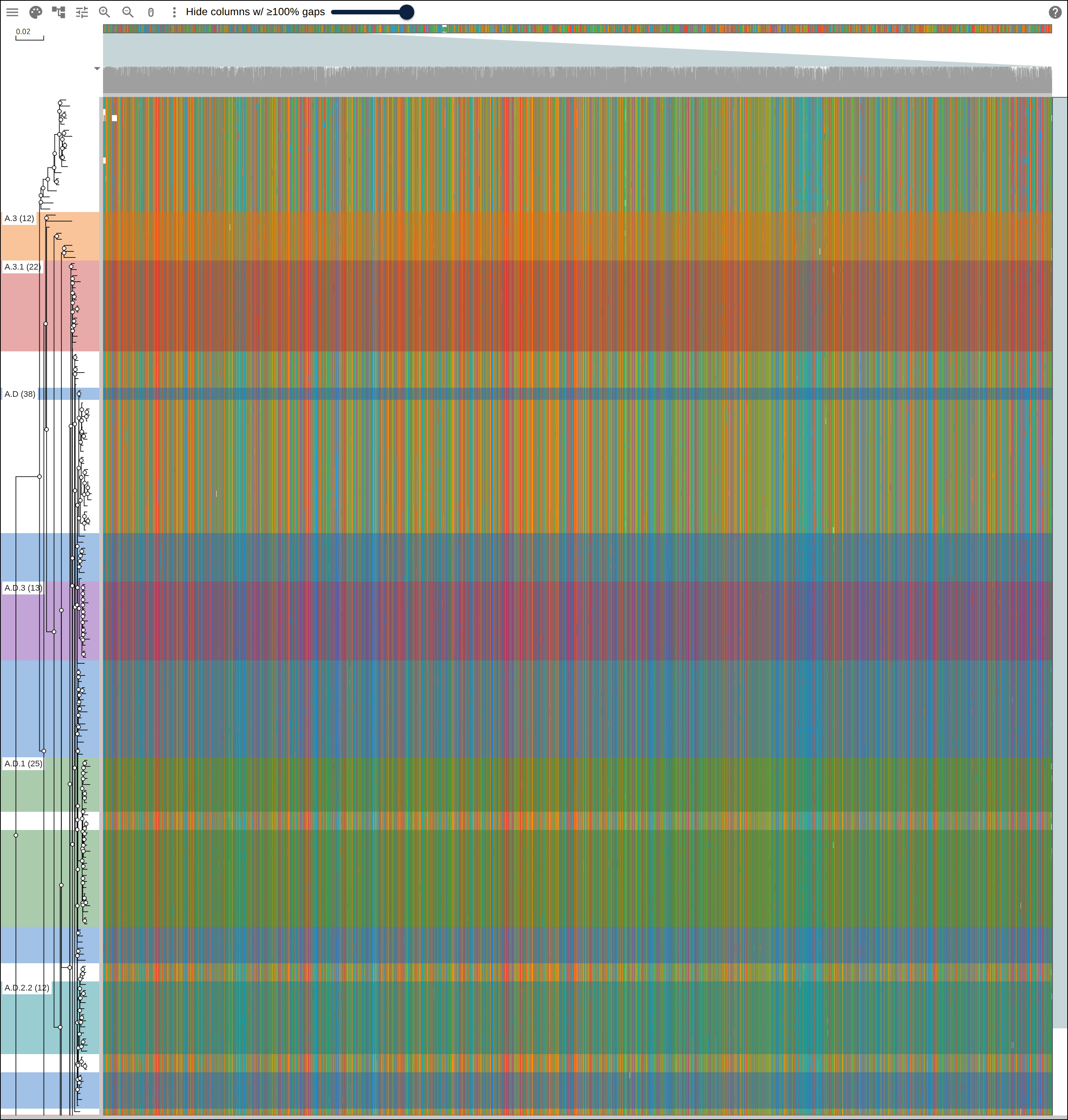
Each tip’s name carries its clade, so the names in the hosted file give the rows
of each clade. A highlights entry for each of the six largest clades tints
their rows as bands without reordering them.
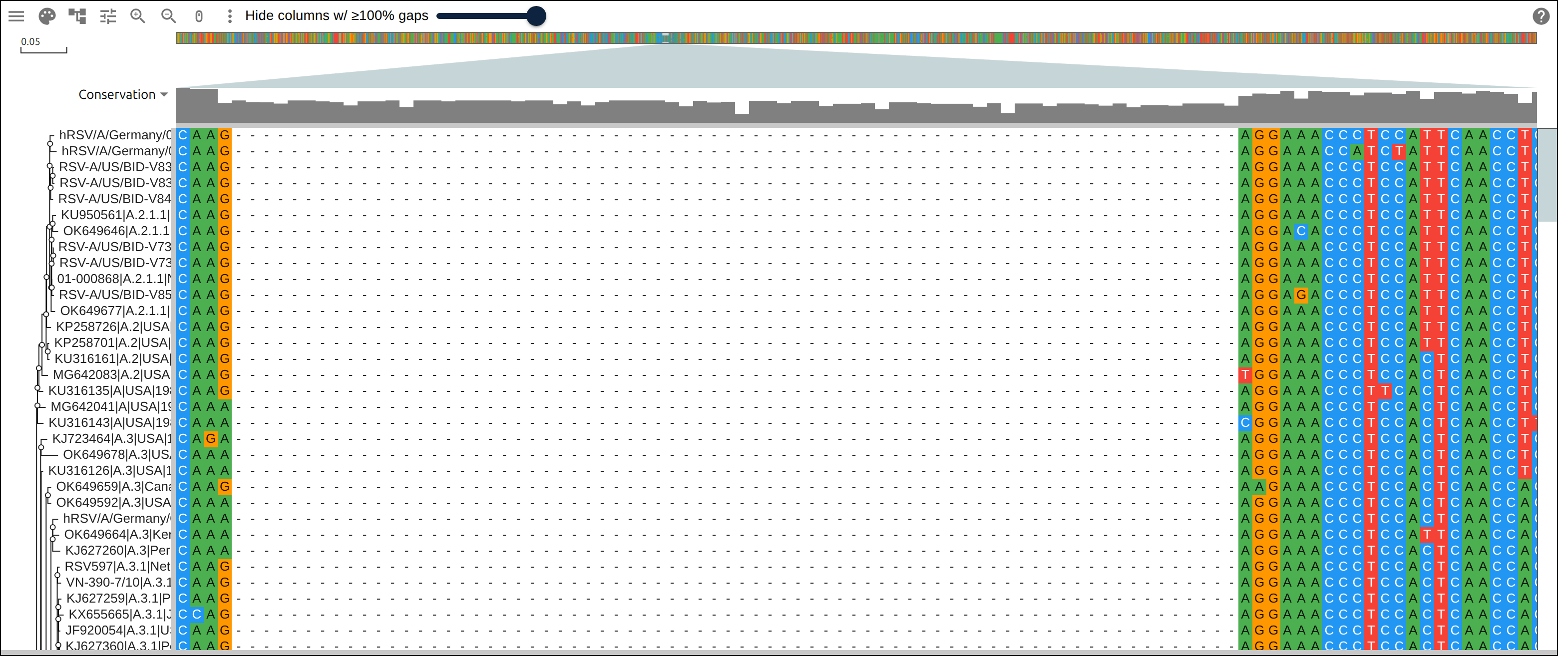
6. Zoom in on the variable end#
This view is at base resolution over columns 5442-5541, inside the G ectodomain, where every one of the 100 columns varies somewhere in the subsample.
7. Zoom in on the conserved end#
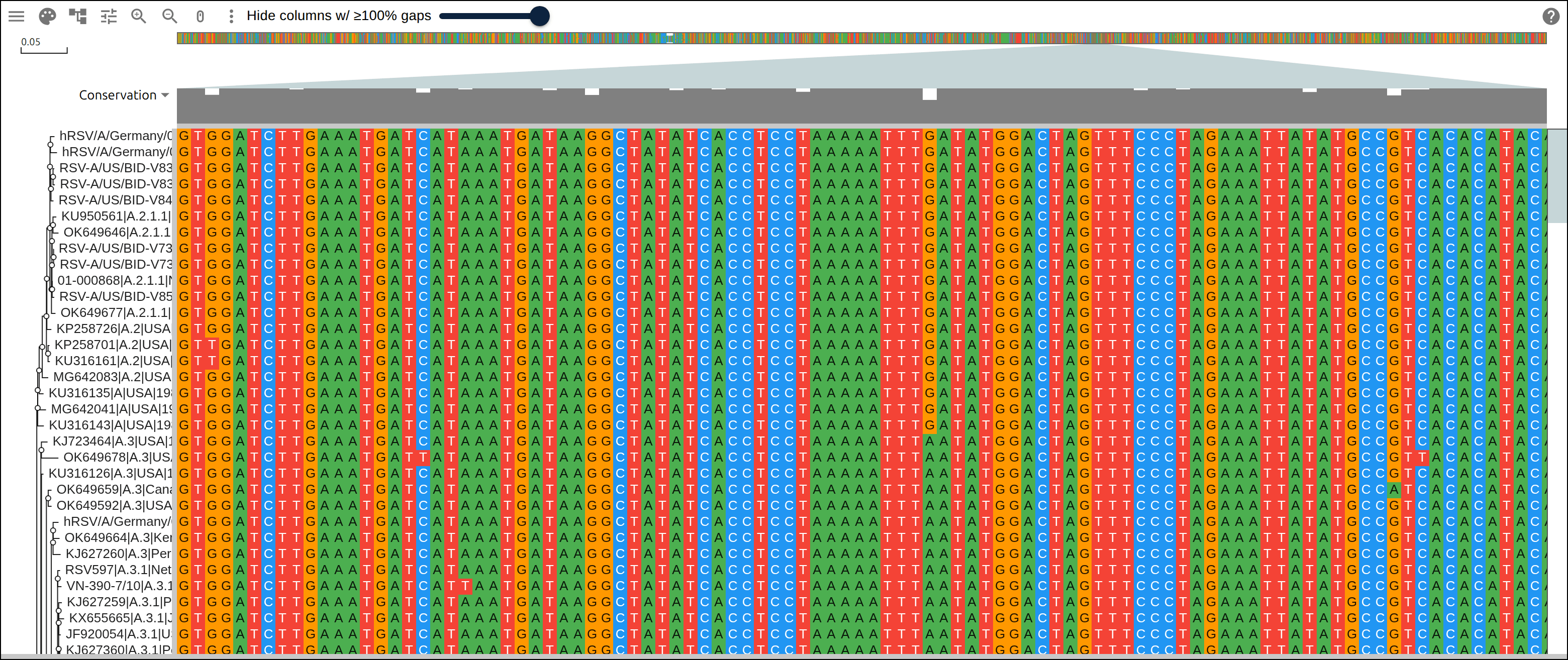
The same view scrolled to columns 10132-10231, inside L.
Check the counts#
The build script counts, over each whole gene of the subsampled alignment and over the two 100-column windows above, how many columns hold more than one letter:
def variable_columns(seqs, start1, end1):
    count = 0
    for col in range(start1 - 1, end1):
        alleles = {s[col] for s in seqs} - {"N"}
        count += len(alleles) > 1
    return count
G gene: 612/966 variable columns (63.4%)
L gene: 1802/6498 variable columns (27.7%)
G hotspot (5442-5541): 100/100 variable columns
L coldspot (10132-10231): 15/100 variable columnsOver each whole gene, G is more than twice as variable as L: 63.4% of its columns differ somewhere in the subsample, against 27.7% of L’s.
Reproduce it end to end#
curl -O https://raw.githubusercontent.com/GMOD/JBrowseMSA/main/docs/tutorials/scripts/build_phylogeny_at_scale.sh
bash build_phylogeny_at_scale.sh
With no arguments the script fetches the Nextstrain build, writes the four files above beside it, and prints every number on this page.
See also#
- Coloring an RSV phylogeny by its metadata
- A protein family from a list of accessions
- User guide
- Data layers
References#
- Hadfield J, Megill C, Bell SM, et al. Nextstrain: real-time tracking of pathogen evolution. Bioinformatics 34:4121-4123.
- Johnson PR, Spriggs MK, Olmsted RA, Collins PL. The G glycoprotein of human respiratory syncytial viruses of subgroups A and B: extensive sequence divergence between antigenic subgroups. Proc Natl Acad Sci USA 84:5625-5629.
- Goya S, Galiano M, Nauwelaers I, et al. Toward unified molecular surveillance of RSV: a proposal for genotype definition and nomenclature harmonized with WHO clinical severity groups. Influenza Other Respir Viruses 14:274-285.