An H5N1 surveillance figure
Nextstrain’s H5N1 cattle-outbreak build places 5,608 genomes on one tree and records a host, a collecting state, a collection date and a GenoFLU genotype for each of them. This page subsamples that build to 204 genomes, writes those fields and one amino-acid site per segment out as a row table, and composes the result into one figure: tip labels and tree edges colored by state, nine strips between the tree and the alignment, three groups marked in the gutter, a collapsed clade, and the whole tree in an overview band above the view. Every layer is a property of the view, so the finished figure is one link and one SVG export.
Prerequisites#
- Python 3, standard library only, nothing to install
- nothing to read along: every figure below links to the live view it captured
Where the data comes from#
One dated Nextstrain build, plus the three files this page writes from it.
- the build every field and every sequence comes from, pinned to 2026-09-15: https://nextstrain.org/avian-flu/h5n1-cattle-outbreak/genome@2026-09-15
- the HA alignment this page writes, 204 rows: https://gmod.org/JBrowseMSA/demo/data/h5n1/h5n1-ha.fa
- its tree: https://gmod.org/JBrowseMSA/demo/data/h5n1/h5n1.nwk
- the row table: https://gmod.org/JBrowseMSA/demo/data/h5n1/h5n1-rowdata.json
1. The build, and the sample#
The auspice JSON holds a root sequence and one mutation list per branch. Copying the root down the tree and applying each branch’s mutations reconstructs every tip, and Nextstrain numbers every mutation against the same reference, so the tips come out already aligned:
def apply_muts(seq, muts):
    edited = bytearray(seq)
    for mut in muts or []:
        m = MUT_RE.match(mut)
        if m:
            _, pos, alt = m.groups()
            edited[int(pos) - 1] = ord(alt)
    return bytes(edited)
The sample is every 24th tip whose record names a GenBank accession and a collecting state, which keeps the proportions of the whole build with no seed to explain:
python3 build_influenza_surveillance_figure.py .build updated 2026-09-14, genome 13590 nt
reconstructed 5608 tips
data source: {'genbank': 4879, 'sra-via-andersen-lab': 729}
4878 tips have a GenBank accession and a reported state
sample: every 24th of them, 204 tips
genotype: 1 values (B3.13 204)
host: 4 values (Cattle 177, Avian 16, Nonhuman Mammal 7, Human 4)
state: 16 values (California 111, Idaho 34, Texas 15, Colorado 14)
year: 3 values (2024 139, 2025 57, 2026 8)
cleavage site: 3 values (RRKR 185, RKKR 18, RRRR 1)All 204 tips carry the same GenoFLU genotype, B3.13, because the build is the cattle outbreak and GenoFLU names a genotype by its eight segment lineages. A strip over that field would draw one color for every row, so the figure reads an amino-acid site per segment instead.
2. The row table#
For each segment’s gene the script takes the amino-acid site whose minor state the most sampled tips carry:
for i in range(length):
    states = collections.Counter(
        chr(t["aa"][gene][i]) for t in sample if i < len(t["aa"][gene])
    )
    called = [(n, s) for s, n in states.items() if s not in ("X", "-")]
    if len(called) < 2:
        continue
    called.sort(reverse=True)
    minor = sum(n for n, _s in called[1:])
PB2 670: R 134, K 70
PB1 517: I 195, V 9
PA 432: I 137, V 66, T 1
HA 147: V 117, M 86, I 1
NP 119: V 138, I 66
NA 71: S 177, N 25, X 1, I 1
M1 82: N 138, S 66
NS1 67: G 138, R 66Each site becomes a field named for its gene and its position, so a strip’s header names what its column reads. The five metadata fields and the eight segment sites go into one file keyed by tip name:
wrote ./h5n1-rowdata.json: 204 rows, 53 kB
the eight segment columns hold 10 states: G I K M N R S T V X
wrote ./h5n1-ha.fa: 204 rows, 1707 columns (HA 6937-8643 of the genome), 348 kB
wrote ./h5n1.nwk: 204 tips, 149 internal nodes, 352 edges
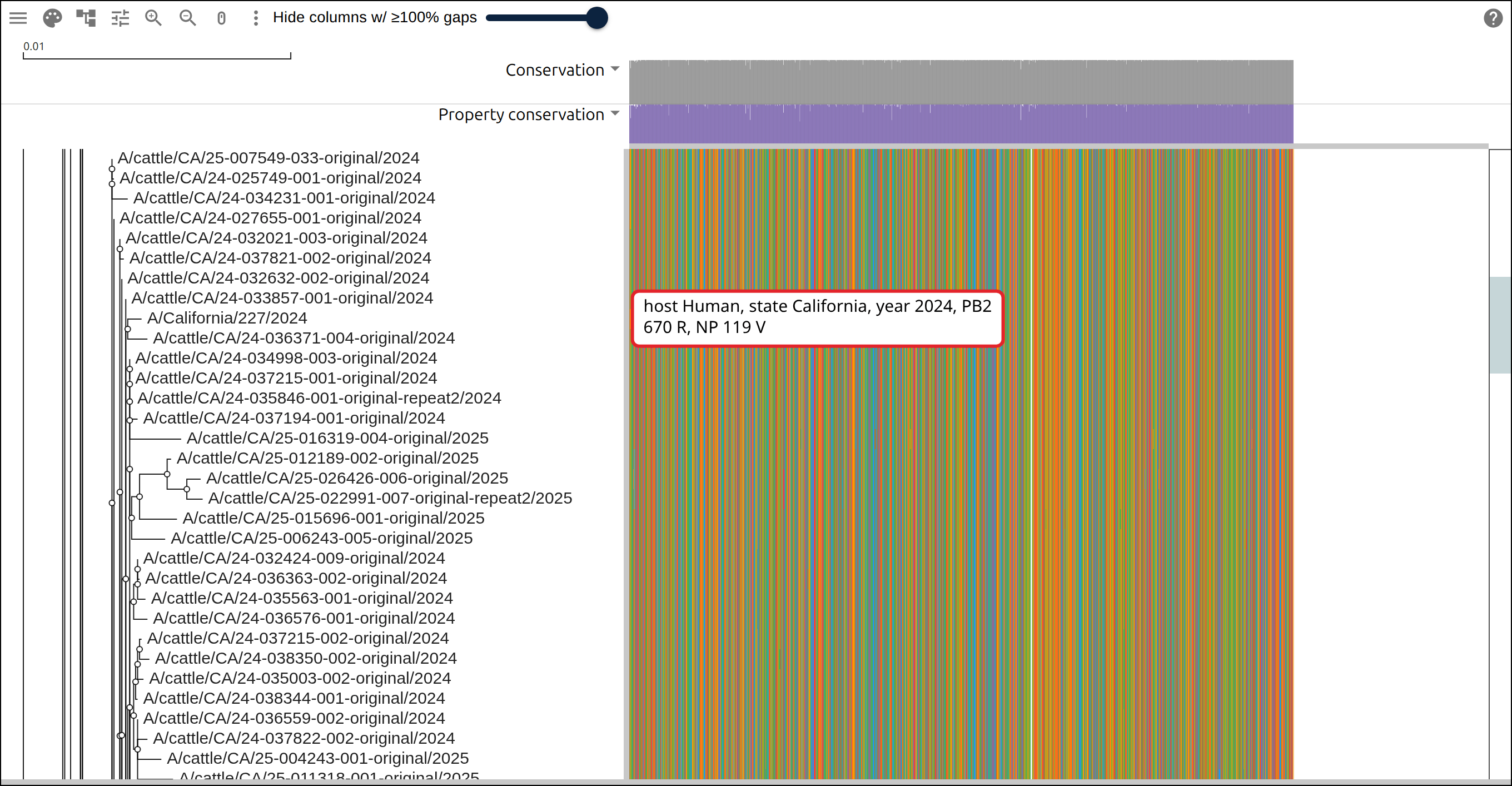
The alignment is the HA coding sequence cut out of each reconstructed genome at the coordinates the build annotates. The tree is the build’s own topology pruned to the 204 tips, with each surviving branch’s length taken from the difference in cumulative divergence. Nextstrain infers that topology with IQ-TREE and publishes a divergence and an inferred date per node, so the Newick written here carries no support values on its internal nodes. A 53 kB table runs past the 8,192-character request line a link fits in, so the snapshot names the three files and the viewer fetches them at startup:
{
  "type": "MsaView",
  "msaFilehandle": { "uri": "data/h5n1/h5n1-ha.fa" },
  "treeFilehandle": { "uri": "data/h5n1/h5n1.nwk" },
  "treeMetadataFilehandle": { "uri": "data/h5n1/h5n1-rowdata.json" }
}
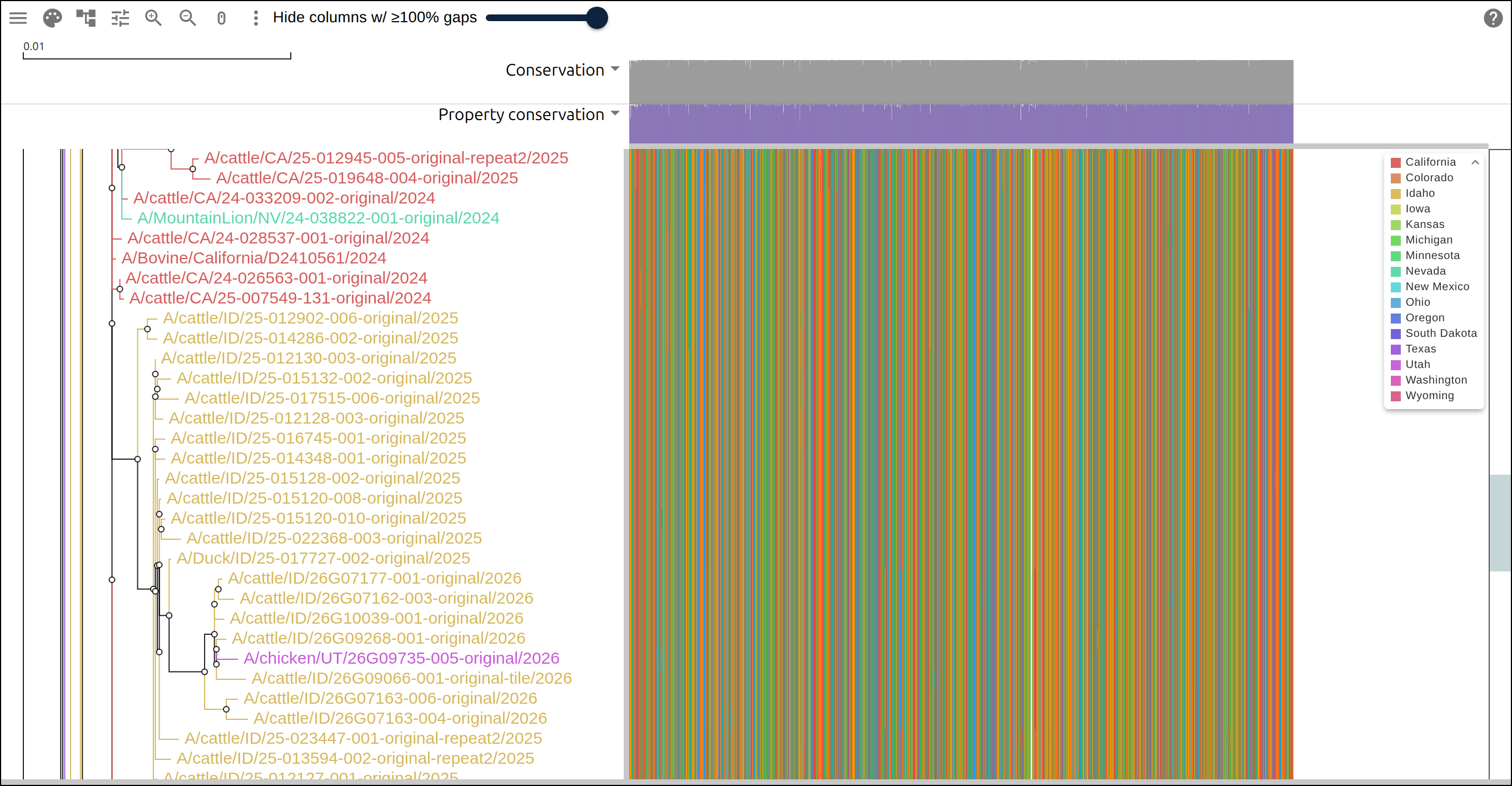
3. Labels and branches colored by state#
An encodings record names the channel to paint and the field feeding it. The
tipLabel channel colors the label beside each tip, and the branch channel
gives an internal node the field value its tips agree on and colors the edge
above it:
"encodings": [
  { "channel": "tipLabel", "field": "state" },
  { "channel": "branch", "field": "state" }
]
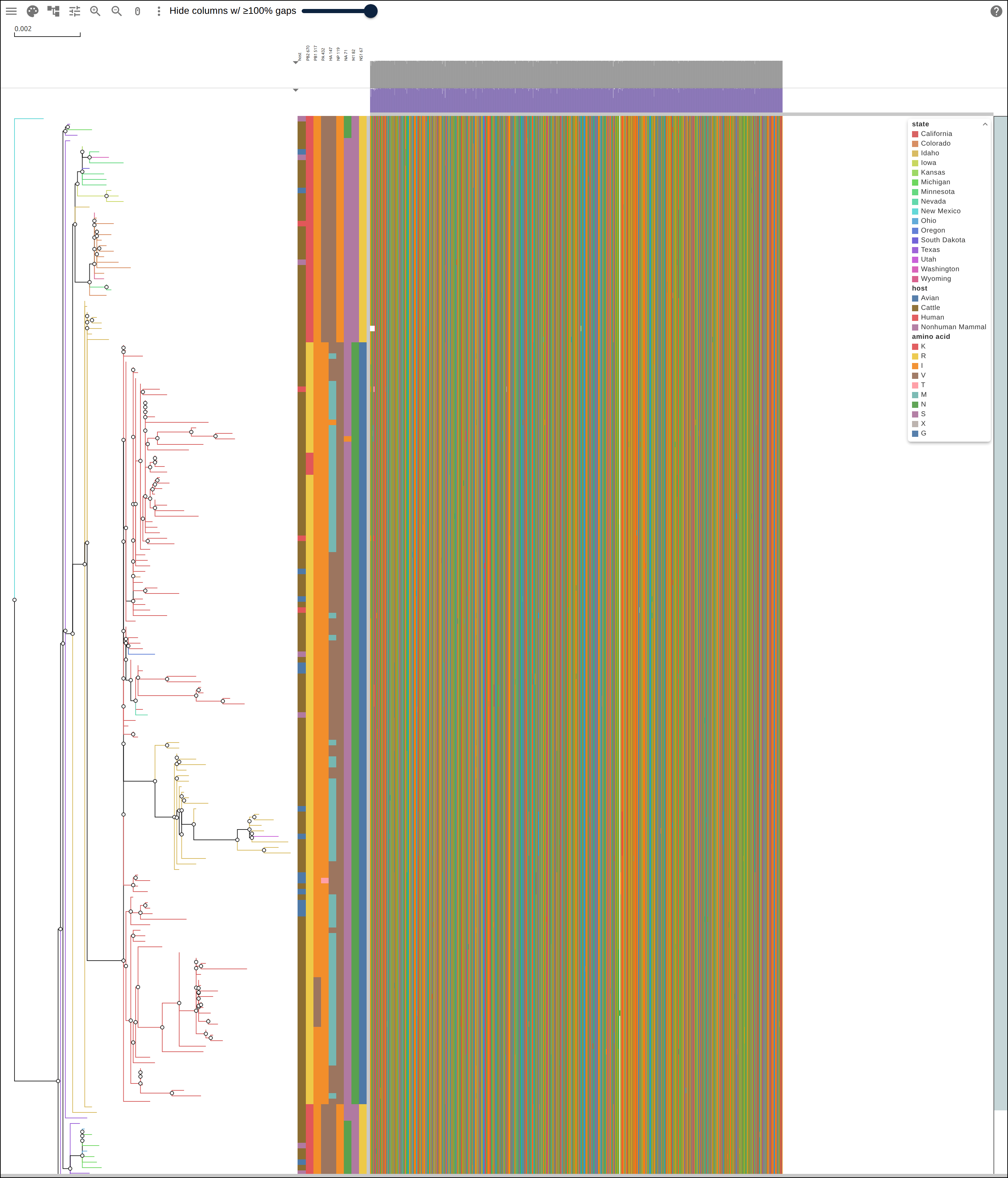
4. Nine strips between the tree and the alignment#
A rowPanels record draws a column of cells, one per row, in the space between
the tree and the alignment. The host field takes one strip and the eight segment
sites take eight more, all nine sharing a color map over amino acids so a state
keeps its color across the matrix:
{
  "kind": "strip",
  "field": "PB2 670",
  "width": 11,
  "legend": "amino acid",
  "scale": {
    "map": {
      "G": "#4e79a7",
      "I": "#f28e2b",
      "K": "#e15759",
      "M": "#76b7b2",
      "N": "#59a14f",
      "R": "#edc948",
      "S": "#b07aa1",
      "T": "#ff9da7",
      "V": "#9c755f",
      "X": "#bab0ac"
    }
  }
}
The other seven segment strips repeat that record with their own field. The
host strip takes a map of its own over the four host values, at a width of 12.
legend names the legend a strip lists under. All eight segment strips name the
same one, so the ten amino-acid states are listed once instead of eight times.
5. How far a field follows the tree#
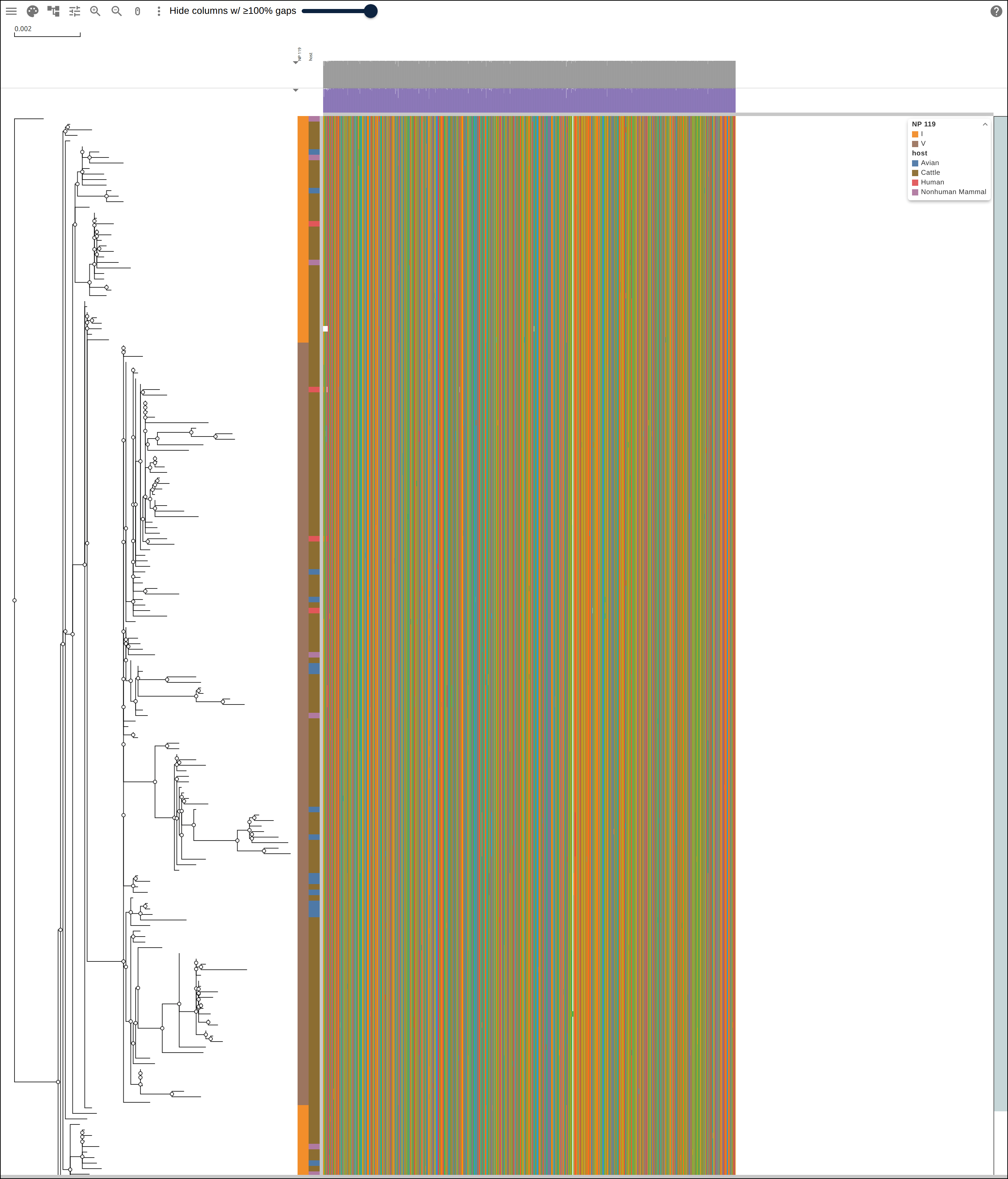
The build script counts, for each field, how many edges take a color and how many maximal clades the field’s values cut the tree into. A field that follows the tree perfectly has one clade per value. Each line the script prints goes on to name the largest clades per value, and the block below stops at the edge counts:
host: 4 values in 112 clades, 285/352 edges colored, 81/148 of them above an internal node
state: 16 values in 86 clades, 297/352 edges colored, 93/148 of them above an internal node
NP 119: 2 values in 15 clades, 345/352 edges colored, 141/148 of them above an internal node
M1 82: 2 values in 15 clades, 345/352 edges colored, 141/148 of them above an internal node
NS1 67: 2 values in 15 clades, 345/352 edges colored, 141/148 of them above an internal node
Two strips put the two extremes side by side: NP 119, whose two states cut the tree into 15 clades, and host, whose four values cut it into 112.
6. Three groups marked in the gutter#
A clades record marks a group of rows. mrca names two tips whose common
ancestor is the group and tips is the leaf count the producer measured under
that ancestor; range names the first and last row of a run that is not a
clade. highlight fills the rows, and bracket draws a bar with the record’s
label in the gutter at the right of the tree area:
"clades": [
  {
    "mrca": ["A/cattle/CA/24-027807-002-original/2024", "A/chicken/CA/24-031285-004-original/2024"],
    "tips": 138,
    "mark": "bracket",
    "color": "#a16207",
    "label": "NP 119V, 138"
  },
  {
    "range": ["A/cattle/ID/25-012902-006-original/2025", "A/cattle/ID/26G09268-001-original/2026"],
    "tips": 17,
    "mark": "bracket",
    "color": "#1d4ed8",
    "label": "Idaho, 17"
  }
]
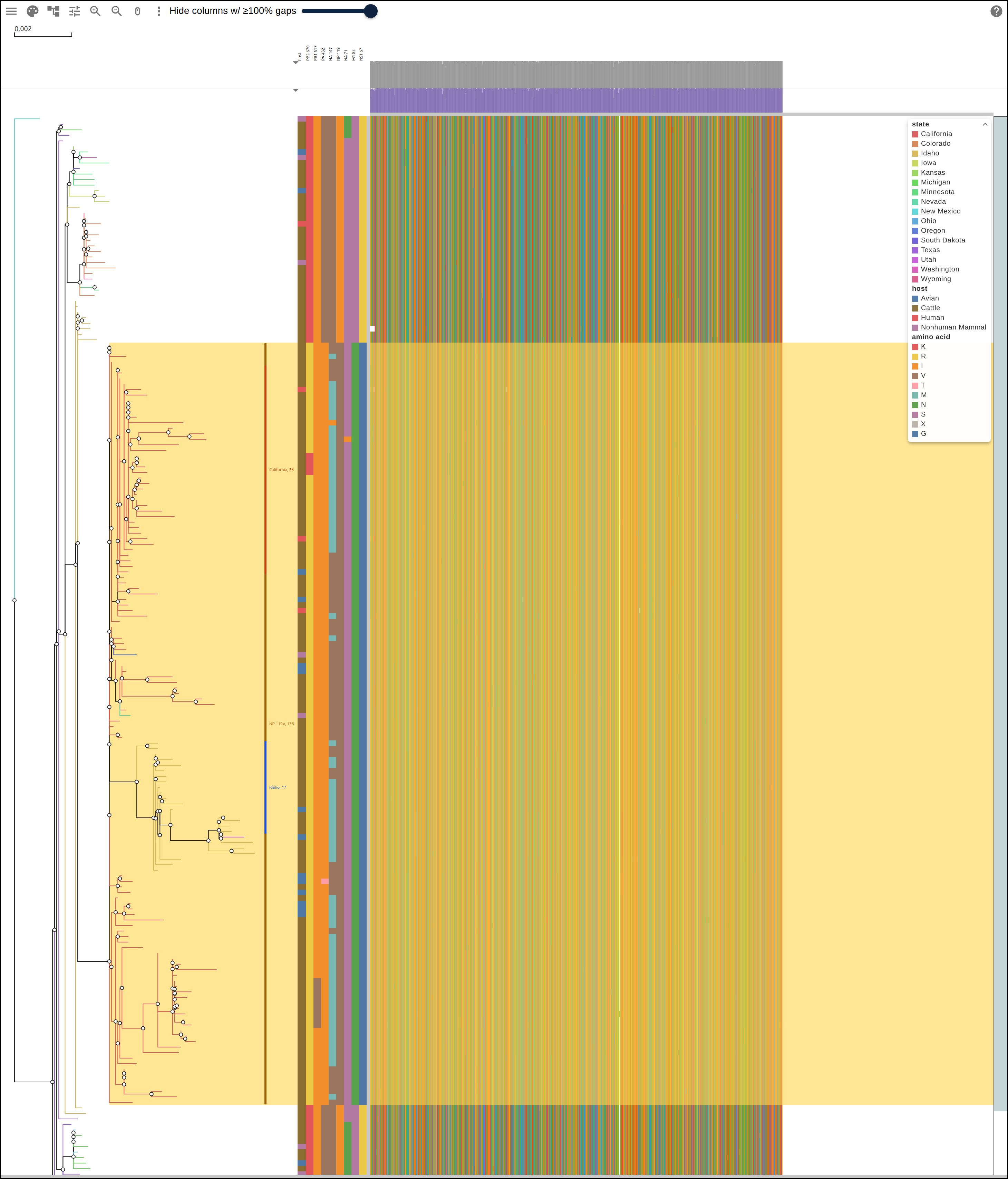
The script finds all three groups on the pruned tree:
NP 119 I->V: a clade of 138 tips, display rows 41-178
  mrca tips: A/cattle/CA/24-027807-002-original/2024 and A/chicken/CA/24-031285-004-original/2024
largest all-California clade: 38 of the 111 California tips, display rows 45-82
  mrca tips: A/chicken/CA/24-031667-001-original/2024 and A/cattle/CA/24-037821-002-original/2024
  longest run of Idaho rows: 17 rows 113-129, not a clade
  range ends: A/cattle/ID/25-012902-006-original/2025 and A/cattle/ID/26G09268-001-original/2026
The same 138 tips carry NP 119V, M1 82N and NS1 67G, so one bracket covers all
three sites. The viewer resolves each mrca pair to their common ancestor,
counts the leaves under it and compares the count with the record’s tips.
Writing 137 there drops the mark, so a re-estimated tree loses it rather than
moving it somewhere else.
range.7. Collapsing a clade#
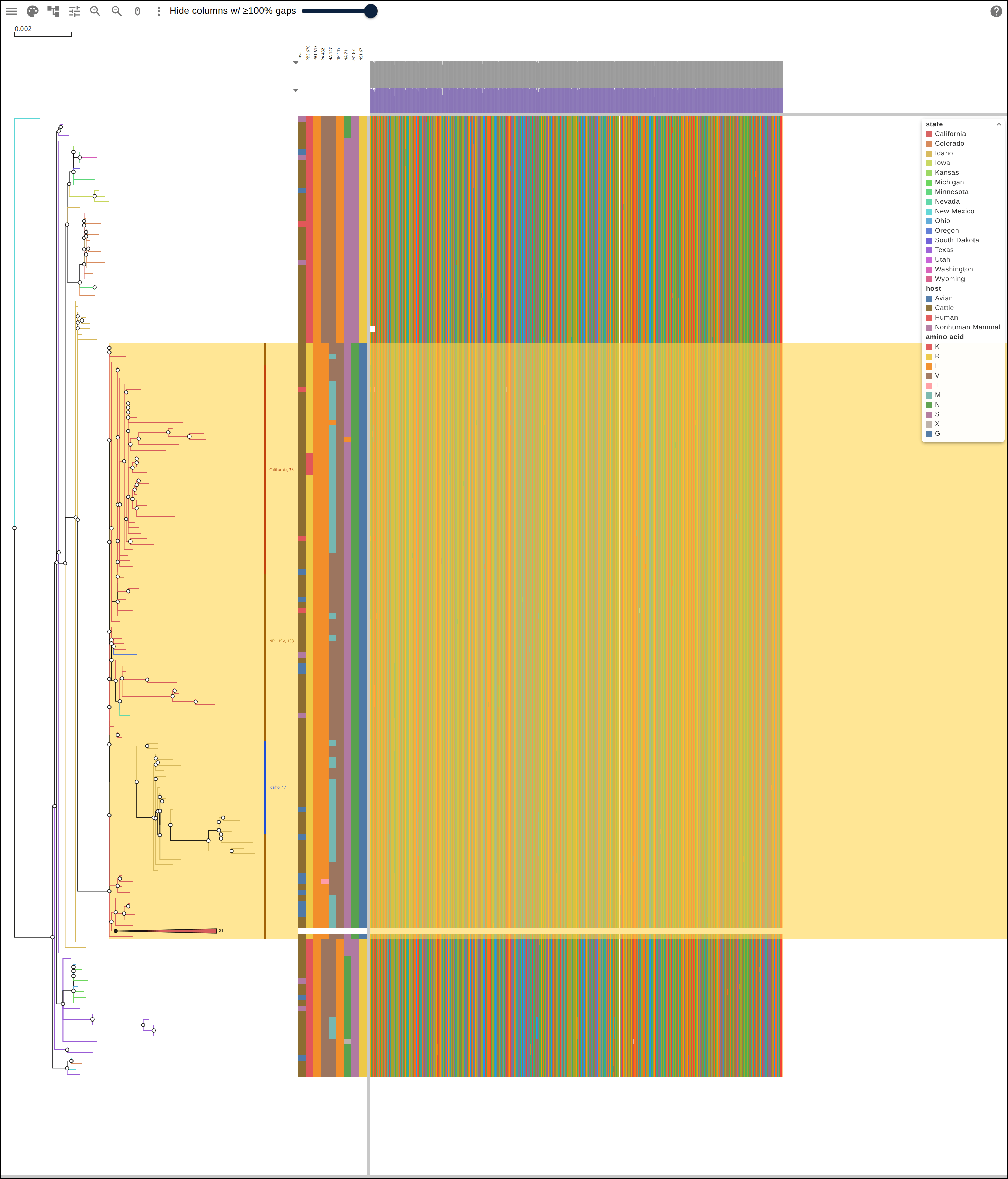
A collapse mark folds a clade into one triangle, and the alignment loses the
same rows. The script takes the largest node whose tips share one state and one
host:
collapse target: 31 tips, all Cattle from California, display rows 147-177
  mrca tips: A/cattle/CA/24-034698-001-original/2024 and A/cattle/CA/24-037190-002-original/2024
{
"mrca": [
"A/cattle/CA/24-034698-001-original/2024",
"A/cattle/CA/24-037190-002-original/2024"
],
"tips": 31,
"mark": "collapse"
}
8. The overview band#
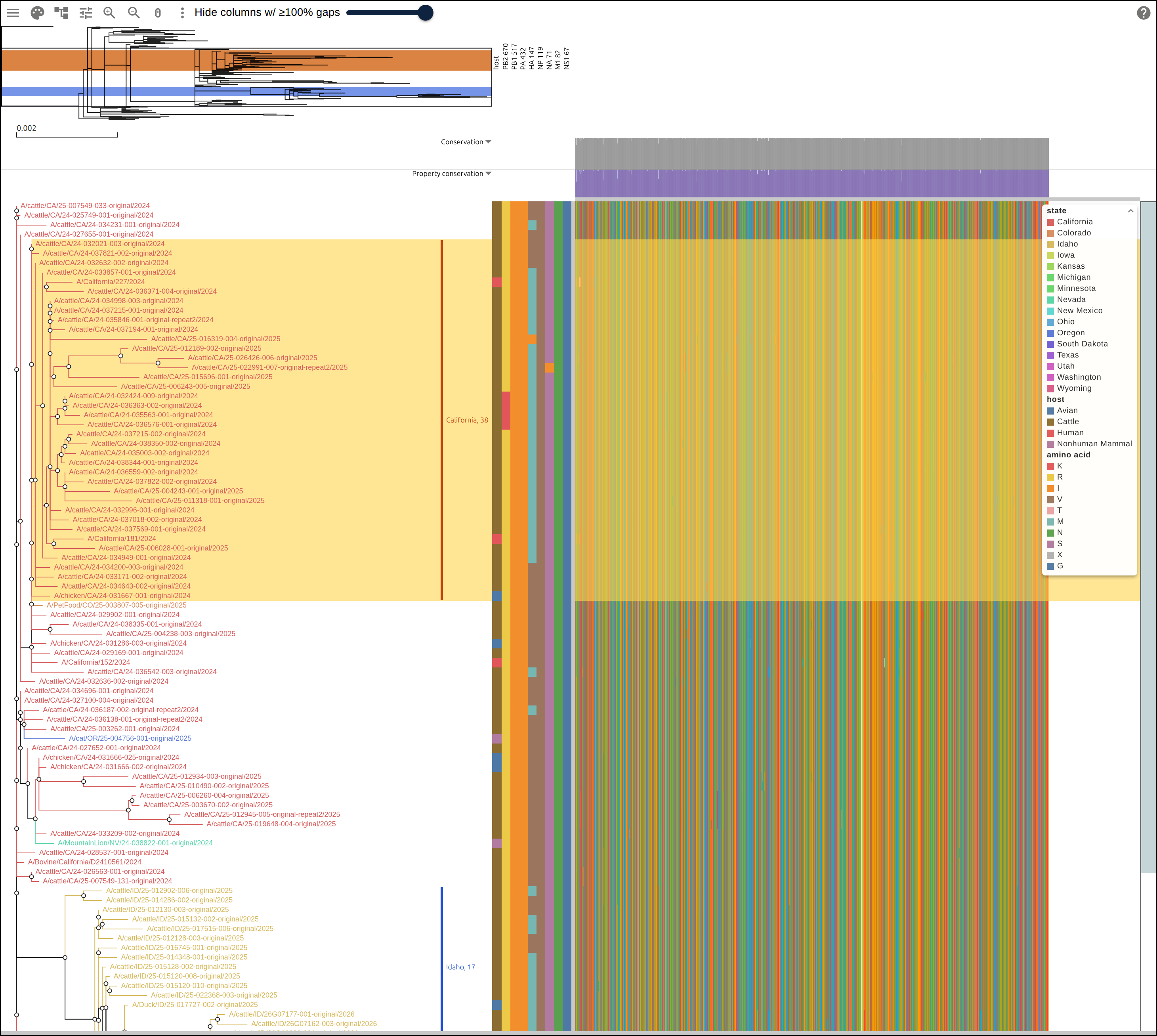
showTreeOverview draws the whole tree in the band above the tree panel, with
the clade highlights in place and a box around the rows the view shows. A
focus mark seeds the view with one subtree, so the alignment shows 138 of the
204 rows while the band keeps drawing all 204:
{
  "mrca": [
    "A/cattle/CA/24-027807-002-original/2024",
    "A/chicken/CA/24-031285-004-original/2024"
  ],
  "tips": 138,
  "mark": "focus"
}
9. The link, the export, and one row read against the build#
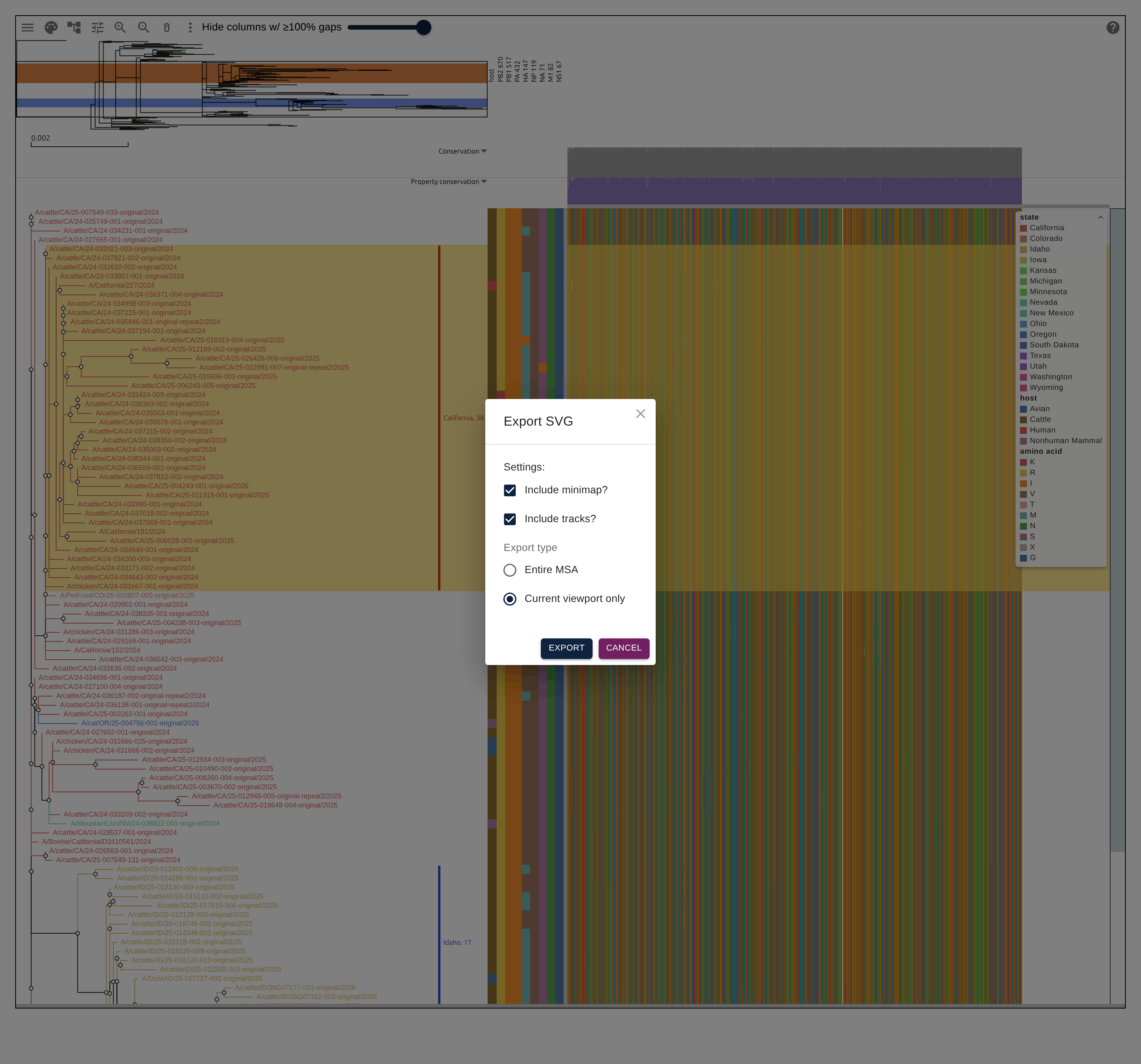
Every layer above is a property of the view, so the whole figure travels in one link: three filehandles, two encodings, nine row panels and four clade records. Export SVG in the file menu writes the same figure as vector graphics, with the overview band, the strips, the bracket labels, the legends and the scale bar each drawn by the same code the screen uses.
The script ends by printing the most recent human case in the sample beside the build’s own record for it:
check tip: A/California/227/2024, display row 49
  node_attrs: {"genbank_accession": {"value": "PX279438"}, "genoflu": {"value": "B3.13"}, "host": {"value": "Human"}, "division_metadata": {"value": "California"}, "num_date": {"value": 2024.958, "confidence": [2024.958, 2024.958], "inferred": false}, "cleavage_site_sequence": {"value": "RRKR"}}
  row: {"genotype": "B3.13", "host": "Human", "state": "California", "year": "2024", "cleavage site": "RRKR", "PB2 670": "R", "PB1 517": "I", "PA 432": "I", "HA 147": "M", "NP 119": "V", "NA 71": "S", "M1 82": "N", "NS1 67": "G"}
  PB2 670: R (root K)
  PB1 517: I (root I)
  PA 432: I (root V)
  HA 147: M (root V)
  NP 119: V (root I)
  NA 71: S (root N)
  M1 82: N (root S)
  NS1 67: G (root R)
On screen that row sits at display row 49, inside the amber rectangle whose 138 tips carry NP 119V, and its host strip reads the red of Human. Seven of its eight segment sites differ from the root state, and the one that matches, PB1 517 I, is the site whose minor state only 9 of the 204 tips carry.
The state field the strip and the two channels read is division_metadata, the
state the record itself reports. The build also carries a division field,
which is the state Nextstrain infers for a tip whose record names none. An
inferred value follows the tree by construction, so a strip over it would answer
the question step 5 asks before the data did.
Reproduce it end to end#
curl -O https://raw.githubusercontent.com/GMOD/JBrowseMSA/main/docs/tutorials/scripts/build_influenza_surveillance_figure.py
python3 build_influenza_surveillance_figure.py .
The argument is the directory to work in. The script fetches the pinned build
there, writes h5n1-ha.fa, h5n1.nwk and h5n1-rowdata.json beside it, and
prints every number on this page. The pin makes a rerun write the same files, so
the row indices and tip names in the snapshots above keep resolving.
The build is assembled from GenBank and SRA. The per-segment builds that carry a
GenoFLU lineage per tip, avian-flu/h5n1/<segment>/2y, draw on GISAID as well,
and the GISAID database access agreement does not allow those sequences to be
redistributed, so this page stays on the GenBank-and-SRA build.
See also#
- Coloring an RSV phylogeny by its metadata
- An RSV phylogeny from a public Nextstrain build
- Data layers
- User guide
References#
- Hadfield J, Megill C, Bell SM, et al. Nextstrain: real-time tracking of pathogen evolution. Bioinformatics 34:4121-4123.
- Minh BQ, Schmidt HA, Chernomor O, et al. IQ-TREE 2: new models and efficient methods for phylogenetic inference in the genomic era. Mol Biol Evol 37:1530-1534.
- Yu G, Smith DK, Zhu H, Guan Y, Lam TT. ggtree: an R package for visualization and annotation of phylogenetic trees with their covariates and other associated data. Methods Ecol Evol 8:28-36.