GMOD
Chado Tutorial 2013
(Redirected from Chado Tutorial
This Chado tutorial was presented by Scott Cain as part of the 2013 GMOD Summer School.
Chado is the database schema of the GMOD project. This session introduces database concepts, and then provides an overview of Chado’s design and architecture, and then goes into detail about how to use a Chado database.
Contents
- 1 Theory
- 2 Practice
- 3 Chado for Expression, Genotype, Phenotype, and Natural Diversity
Theory
Introduction
Database Terminology
Or six years of school in 15 minutes or less.
What’s a database?
- Chado is a schema, a database design - a blueprint for a database containing genomic data
- Distinct from
- Database Management System
(DBMS)
- Software system for storing databases
- e.g., Oracle, PostgreSQL, MySQL
- Database, a very loose term
- Any set of organized data that is readable by a computer
- A web site with database driven content, e.g., FlyBase
- Schema + DBMS + Data
- Database Management System
(DBMS)
SQL
SQL is a standardized query language for defining and manipulating databases. Chado uses it. SQL is supported by all major DBMSs.
FlyBase Field Mapping Tables shows some example SQL that queries the FlyBase Chado database. (Caveat: FlyBase sometimes uses Chado in ways that no other organizations do.)
Will SQL be on the test?
No, we aren’t going to teach in-depth SQL in this course but we will use it in examples and show how to write queries in Chado.
You can do basics with Chado without knowing SQL. Many common tasks already have scripts written for them. However, as you get more into using Chado, you will find that a working knowledge of SQL is necessary.
Why Chado?
- Integration
- Supports many types of data, integrates with many tools
- Modular
- Use only what you need, ignore the rest
- Extensible
- Write your own modules and properties
- Widely used
- FlyBase - Chado started here, large diverse dataset and organization
- Xenbase - Smaller, but with several IT staff
- ParameciumDB - Smaller still, complete GMOD shop, including Chado
- IGS - Large-scale annotation/comparative data in Chado, more than a dozen active developers
- Plus AphidBase, BeeBase, BeetleBase, BovineBase, …
- Great Community of Support
Chado Architecture: Modules
The Chado schema is built with a set of modules. A Chado module is a set of database tables and relationships that stores information about a well-defined area of biology, such as sequence or attribution.
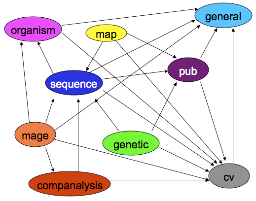
(Also available as a PowerPoint animation)
Arrows are dependencies between modules. Dependencies indicate one or more foreign keys linking modules.
- General - Identifying things within the DB to the outside world, and identifying things from other databases.
- Controlled Vocabulary (cv) - Controlled vocabularies and ontologies
- Publication (pub) - Publications and attribution
- Organism - Describes species; pretty simple. Phylogeny module stores relationships.
- Sequence - Genomic features and things that can be tied to or descend from genomic features.
- Map - Maps without sequence
- Genetic - Genetic data and genotypes
- Companalysis - Storage of Computational sequence analysis. The key concept is that the results of a computational analysis can be interpreted or described as a sequence feature.
Extensible
These modules have been contributed to Chado by users who developed them.
- Mage - Microarray data
- Stock - Specimens and biological collections
- Natural Diversity - geolocation, phenotype, genotype
- Plus property tables in many modules.
Plus
- Audit - Database audit trail
- Expression - Summaries of RNA and protein expression
- Library - Descriptions of molecular libraries
- Phenotype - Phenotypic data
- Phylogeny - Organisms and phylogenetic trees
Module Caveats
All modules are blessed, but some modules are more blessed than others.
The General, CV, Publication, Organism, Sequence and Companalysis modules are all widely used and cleanly designed. After that modules become less frequently used (Stock, Expression, Phenotype, Mage). Also several modules are not as cleanly separated as we would like them to be. Phenotypic data is spread over several modules. Organism and Phylogeny overlap. CMap is all about maps, but it does not use the Map module.
From Jeff Bowes, at XenBase:
As for Chado, we are more Chadoish than exactly Chado. We use the core modules with few changes - feature, cv, general, analysis. Although I prefer to add columns to tables when it is reasonable and limit the use of property tables (too many left outer joins). We use a slightly modified version of the phylogeny module. We have developed completely different modules for community, literature, anatomy and gene expression. If there is a PATO compatible Chado Phenotype solution we’d prefer to go with that. Although, it might cause problems that we have a separate anatomy module as opposed to using cvterm to store anatomy.
In other words the ideal is good, but implementation and usage is uneven. See the 2008 GMOD Community survey for what gets used.
Exploring the schema
Rather than simply listing out the modules and what is stored in them, we’ll take a data-centric view and imagine what we want to store in our database, then learn the Chado way of storing it.
During this course you’ll be working with genome annotation data from MAKER. We’ll simplify this and start by considering that we have annotation on chromosomes that we want to store in our database. These are the sort of things we want to store:
- chromosomes
- genes
- gene predictions
- tRNAs
- BLAST matches
You may have worked with databases in the past where each type of thing you want to store is given its own table. That is, we’d have a table for genes, one for chromosomes, tRNAs, etc. The problem with this sort of design is that, as you encounter new types of things, you have to create new tables to store them. Also, many of these ‘thing’ tables are going to look very much alike.
Chado is what is a generic schema which, in effect, means that data are abstracted wherever possible to prevent duplication in both the design and data itself. So, instead of one table for each type of ‘thing’, we just have one table to hold ‘things’, regardless of their types. In the Chado world these are known as ‘features’. (This database design pattern is called the Entity-Attribute-Value model.)
This brings us to the Sequence Module, which contains the central feature table.
Sequence Module
The sequence module is used to manage genomic features.
Features
Chado defines a feature to be a region of a biological polymer (typically a DNA, RNA, or a polypeptide molecule) or an aggregate of regions on this polymer. A region can be an entire chromosome, or a junction between two bases. Features are typed according to the Sequence Ontology (SO), they can be localized relative to other features, and they can form part-whole and other relationships with other features.
Features are stored in the feature table.
| Table: feature | |||||
|---|---|---|---|---|---|
| feature_id | name | uniquename | type_id | is_analysis | … |
Within this feature table we can store all types of features and keep track of their type with the type_id field. It’s conceivable to store the named value of each type in this field, like ‘gene’, ‘tRNA’, etc. but this would be prone to things like spelling errors, not to mention disagreement of the definition of some of these terms.
So solve this, all features are linked to a specific type in a controlled vocabulary or ontology. These are stored in the cv module.
CV (Controlled Vocabularies) Module
Controlled Vocabulary Module Tables
The CV module implements controlled vocabularies and their more complex cousins, ontologies.
Controlled Vocabularies
A controlled vocabulary (CV) is a list of terms from which a value must come. CVs are widely used in all databases, not just biological ones. Pull down menus are often used to present CVs to users in query or annotation interfaces.
| | | | — | — |
| ZFIN’s Assay Type CV | 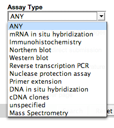 |
|
Ontologies
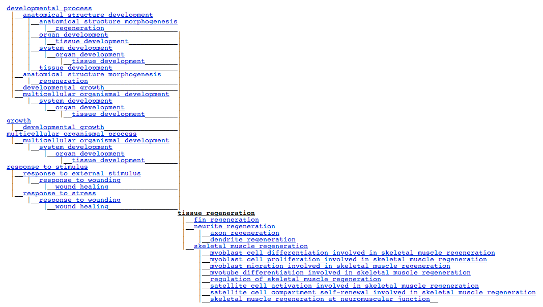
Controlled vocabularies are simple lists of terms. Ontologies are terms plus rules and relationships betwen the terms. The Gene Ontology (GO) and Sequence Ontology (SO) are the two best known ontologies, but there are many more available from OBO.
Ontologies can be incredibly complex with many relationships between terms. Representing them and reasoning with them is non-trivial, but the CV module helps with both.
| FlyBase CV Term Viewer showing GO term “tissue regeneration” |
|—-|
|  |
|
CVs and Ontologies in Chado
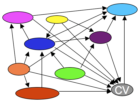
(See the CVTerm table referencing table list.)
Every other module depends on on the CV module. CVs and ontologies are central to Chado’s design philosophy. Why?
Data Integrity
Using CVs (and enforcing their use as Chado does) ensures that your data stays consistent. For example, in the most simple case it prevents your database from using several different values all to mean the same thing (e.g., “unknown”, “unspecified”, “missing”, “other”, “ “,…), and it prevents misspellings (“sagital” instead of “sagittal”) and typos.
Data Portability and Standardization
If you are studying developmental processes and you use the Gene Ontology’s biological process terms then your data can be easily shared and integrated with data from other researchers. If you create your set of terms or just enter free text (egads!), then it will require a lot of human intervention to convert your data to a standard nomenclature so it can be integrated with others.
Using an established ontology when one exists usually involves some compromises, but it greatly increases the usability of your data to others (and to yourself).
Complexity
Controlled vocabularies are not particularly complex - they are just lists of terms. Ontologies, however, can be very complex, as shown by the GO example above. This complexity could be ignored. You could, for example, convert GO to a controlled vocabulary - a very long list of terms. You would still have data integrity and portability, and it wouldn’t be as complex.
It also would not be as powerful. Ontologies support reasoning about the terms in them and this can be very useful. With GO, for example, you can ask
Show me all genes involved in anatomical structure development
and get back genes directly tagged with anatomical structure development, plus any genes tagged with any of that term’s sub-terms, from organ development to regulation of skeletal muscle regeneration. If you convert GO to just a list of terms, you can no longer answer that question.
The Chado CV Module supports such complex queries with ontologies by pre-calculating the transitive closure of all terms in an ontology. There is a great explanation of transitive closure on the Chado CV Module page. Also see the description of these 3 tables:
We won’t go into any more detail on it here.
Opening our sample database
$ psql drupal
Our first example query
Up to this point we’ve seen how to store features using the feature table as well as rigidly define what types of things they are using the cv module tables. Here is an SQL example of how to query some very basic information about all gene features in our database:
 SELECT gene.feature_id, gene.uniquename, gene.name
   FROM feature gene
        JOIN cvterm c ON gene.type_id = c.cvterm_id
  WHERE c.name = 'gene' AND organism_id = 13;
This should return something like:
 feature_id |                   uniquename                   |                      name
------------+------------------------------------------------+------------------------------------------------
        405 | maker-scf1117875582023-snap-gene-0.0           | maker-scf1117875582023-snap-gene-0.0
        409 | maker-scf1117875582023-snap-gene-0.3           | maker-scf1117875582023-snap-gene-0.3
        415 | genemark-scf1117875582023-abinit-gene-0.42     | genemark-scf1117875582023-abinit-gene-0.42
       1011 | maker-scf1117875582023-snap-gene-1.0           | maker-scf1117875582023-snap-gene-1.0
       1018 | maker-scf1117875582023-snap-gene-1.4           | maker-scf1117875582023-snap-gene-1.4
       1022 | maker-scf1117875582023-snap-gene-1.1           | maker-scf1117875582023-snap-gene-1.1
       1027 | maker-scf1117875582023-snap-gene-1.2           | maker-scf1117875582023-snap-gene-1.2
       1032 | maker-scf1117875582023-snap-gene-1.7           | maker-scf1117875582023-snap-gene-1.7
       1038 | maker-scf1117875582023-snap-gene-1.5           | maker-scf1117875582023-snap-gene-1.5
       1698 | snap_masked-scf1117875582023-abinit-gene-2.4   | snap_masked-scf1117875582023-abinit-gene-2.4
...
Type q to escape the listing.
Lists of things are great, but we’re going to need to do a lot more with our genomic data than keep lists of features. First, we need to be able to identify them properly. This may seem straightforward, but creating one column per ID type in feature would be a bad idea, since any given feature could have dozens of different identifiers from different data sources. The General Module helps resolve this.
General Module
The General module is about identifying things within this DB to the outside world, and identifying things from the outside world (i.e., other databases) within this database.
IDs
Biological databases have public and private IDs and they are usually different things.
Public IDs
These are shown on web pages and in publications. These are also known as accession numbers.
| GO + 0043565 = GO:0043565 |
|---|
| InterPro + IPR001356 = InterPro:IPR001356 |
| YourDB + whatever = YourDB:whatever |
Public IDs tend to be alternate keys inside the database: they do uniquely identify objects in the database.
Private IDs
These are used inside the database and are not meant to be shown or published. Tend to be long integers. There are many more private IDs than public IDs.
Private IDs are used for primary keys and foreign keys.
Most DBMSs have built-in mechanisms for generating private IDs.
IDs in Chado
The General module defines public IDs of
- items defined in this databases, and
- items defined in other databases, that are used or referenced in this database.
In fact, those two classes of IDs are defined in exactly the same way, in the dbxref table.
In Chado every table (in every module) defines its own private IDs.
Properties
So far we’ve only seen very basic information for each feature stored. Because the feature table was designed to be very generic and store all feature types, attributes specific to only some types can’t be stored there. It wouldn’t make sense, for example, to have a column called ‘gene_product_name’, since that column would be empty for all the features, like chromosomes, that aren’t gene products.
These feature-specific attributes are known as ‘properties’ of a feature in Chado. They are stored in a table called featureprop.
| Table: featureprop | ||||
|---|---|---|---|---|
| featureprop_id | feature_id | type_id | value | rank |
You may have noticed that the featureprop table shares a ‘type_id’ column with the feature table. Properties of features are typed according to a controlled vocabulary just as the features themselves are. This helps to ensure that anyone using the same vocabularies are encoding their property assertions in the same way.
Using feature properties we can now describe our features as richly as needed, but our features are still independent of one another. Because many of the features we’re storing have some sort of relationship to one another (such as genes and their polypeptide end-products), our schema needs to accommodate this.
Relationships
Relationships between features are stored in the feature_relationship table.
| Table: feature_relationship | |||||
|---|---|---|---|---|---|
| feature_relationship_id | subject_id | object_id | type_id | rank | … |
Features can be arranged in graphs, e.g. “exon part_of transcript part_of gene”; If type is thought of as a verb, then each arc or edge makes a statement:
- Subject verb Object, or
- Child verb Parent, or
- Contained verb Container, or
- Subfeature verb Feature
Again, notice the use of controlled vocabularies (type_id) to define the relationship between features.
One might think of a relationship between a gene and chromosome as ‘located_on’, and store that as a feature_relationship entry between the two. If you did, pat yourself on the back for Chado-ish thinking, but there’s a better way to handle locatable features, since a relationship entry alone wouldn’t actually say WHERE the feature was located, only that it was.
Locations
Location describes where a feature is/comes from relative to another feature. Some features such as chromosomes are not localized in sequence coordinates, though contigs/assemblies which make up the chromosomes could be.
Locations are stored in the featureloc table, and a feature can have zero or more featureloc records. Features will have either
- one featureloc record, for localized features for which the location is known, or
- zero featureloc records, for unlocalized features such as chromosomes, or for features for which the location is not yet known, such as a gene discovered using classical genetics techniques.
- Features with multiple featurelocs are explained below.
(For a good explanation of how features are located in Chado see Feature Locations. This explanation is excerpted from that.)
Interbase Coordinates
This is covered in more detail on the GMOD web site.
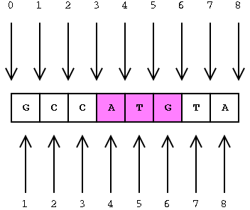
A featureloc record specifies an interval in interbase sequence coordinates, bounded by the fmin and fmax columns, each representing the lower and upper linear position of the boundary between bases or base pairs (with directionality indicated by the strand column).
Interbase coordinates were chosen over the base-oriented coordinate system because the math is easier, and it cleanly supports zero-length features such as splice sites and insertion points.
Location Chains
Chado supports location chains. For example, locating an exon relative to a contig that is itself localized relative to a chromosome. The majority of Chado instances will not require this flexibility; features are typically located relative to chromosomes or chromosomes arms.
The ability to store such localization networks or location graphs can be useful for unfinished genomes or parts of genomes such as heterochromatin, in which it is desirable to locate features relative to stable contigs or scaffolds, which are themselves localized in an unstable assembly to chromosomes or chromosome arms.
Localization chains do not necessarily only span assemblies - protein domains may be localized relative to polypeptide features, themselves localized to a transcript (or to the genome, as is more common). Chains may also span sequence alignments.
featureloc Table
Feature location information is stored in the featureloc table.
| Table: featureloc | |||||
|---|---|---|---|---|---|
| featureloc_id | feature_id | srcfeature_id | fmin | rank | … |
Example: Gene
Note: This example and some of the figures are extracted from A Chado case study: an ontology-based modular schema for representing genome-associated biological information, by Christopher J. Mungall, David B. Emmert, and the FlyBase Consortium (2007)
How is a “central dogma” gene represented in Chado?
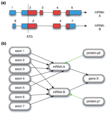
How do we represent these exons, mRNAs, proteins, and there relationships between them?
|
|
||||||||||||||||||||||||||||||||||||||||||||||||||||||||||||||||||||||||||||||||||||||||||||||||||||||||||||||||||||||||||||||||||||||||||||||||||||||||||||||||||||||||||||||
Example: Computational Analysis
Note: This is example is based on an example by Scott Cain from an earlier Chado workshop.
You can store the results of computational analysis such as BLAST or BLAT runs in the sequence module. Here’s an example of you could store a BLAST highest scoring pair (HSP) result.
With HSP results there are two reference sequences, which means two entries in the featureloc table. (The analysis and analysisfeature tables, in the Companalysis module, are used to store information about how the analysis was done and what scores resulted.)
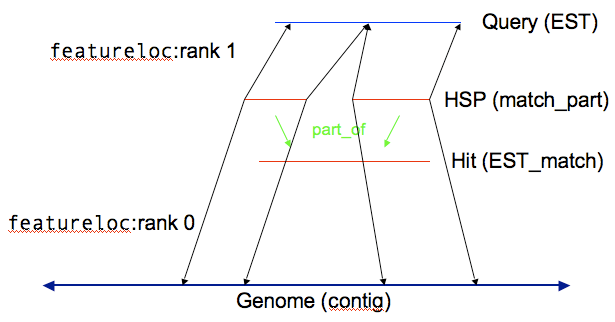
Every horizontal line becomes a record in the feature table, and every vertical line becomes a record in the feature_relationship table.
Other Feature Annotations
Link to any feature via feature_id:
- GO terms in feature_cvterm
- DB links in feature_dbxref
- Miscellaneous features in featureprop
- Attribution in feature_pub
Extending Chado: Properties tables and new modules
Chado was built to be easily extensible. New functionality can be added by adding new modules. Both the Mage and the Stock modules were added after Chado had been out for a while. They both addressed needs that were either not addressed, or were inadequately addressed in the original release.
Chado can be tailored to an individual organization’s needs by using property tables. Property tables are a means to virtually add new columns without having to modify the schema. Property tables are included in many modules.
Property tables are incredibly flexible, and they do make Chado extremely extensible, but they do so at a cost.
- The SQL to get attributes from property tables is much more complex, and
- It is more work to enforce constraints on data in properties tables then in regular columns.
Practice
Prerequisites
Using data from MAKER.
PostgreSQL
Already installed PostgreSQL 9.1 via apt-get.
Edit config files
  sudo su
  cd /etc/postgresql/9.1/main/
  less pg_hba.conf
At the bottom of the file, we’ve already changed ident sameuser to
trust. This means that anyone who is on the local machine is allowed
to connect to any database. If you want to allow people to connect from
other machines, their IP address or a combo of IP address and netmasks
can be used to allow remote access.
If we’d have edited the pg_hba.conf file, we’d have to (re)start the database server:
  /etc/init.d/postgresql restart
  exit # to get out of su
Create a gmod user
Normally, we’d have to switch to the postgres user to create a new database user, but the ubuntu user is already a superuser. Create a new user named “gmod”:
  createuser gmod
    Shall the new role be a superuser? (y/n) y
BioPerl
Version 1.6.901 already installed.
Let’s Go!
Environment Variables
in ~/.bashrc add:
  GMOD_ROOT='/usr/local/gmod'
  export GMOD_ROOT
and source the profile:
source ~/.bashrc
Installing Chado
  cd ~/sources/chado/chado/
  perl Makefile.PL
Use values in '/home/ubuntu/chado/chado/build.conf'? [Y] n
This allows you to specify Pythium when you are asked for a default organism.
 > "chado" for database name
 > "ubuntu" for database username
 > "Pythium" for the default organism
 > "public" for the schema Chado will reside in
Just hit enter when it asks for a password for user gmod.
This Makefile.PL does quite a bit of stuff to get the installation
ready. Among other things it:
- Sets up a variety of database user parameters
- Prepares the SQL files for installation
- It can rebuild Class::DBI api for Chado, but isn’t now (they are prebuilt for the default schema)
- All the ‘normal’ stuff that would happen when running
Makefile.PL, like copyinglibandbinfiles to be ready for installation
 make
 sudo make install
 make load_schema
 make prepdb
At this point, the installer checks the database to see if the organism we put in as our default organism is present in the database. Since it isn’t, it will ask us to add it. It does this by automatically executing a script that comes with Chado, gmod_add_organism.pl. You can execute this script any time you want to add organisms to your database:
 Adding Pythium to the database...

 Both genus and species are required; please provide them below

 Organism's genus?  Pythium
 Organism's species?  ultimum
 Organism's abbreviation? [P.ultimum]
 Comment (can be empty)?
Continuing on…
 make ontologies
 Available ontologies:
 [1] Relationship Ontology
 [2] Sequence Ontology
 [3] Gene Ontology
 [4] Chado Feature Properties
 [5] Plant Ontology

 Which ontologies would you like to load (Comma delimited)? [0]  1,2,4
You can pick any ontologies you want, but GO will take over an hour to install, and it doesn’t matter to much what you pick, because we are going to be blowing this database away soon anyway.
Saving your progress to this point
It is generally a good idea to save your progress when you are done loading ontologies before you’ve attempted to load any other data. That way, if something goes wrong, it is very easy to restore to this point. To make a db dump, do this:
pg_dump chado | bzip2 -c --best > db_w_ontologies.bz2
The -c tells bzip2 to take input on standard in and spit it out on
stdout. To restore from a dump, drop and recreate the database and
then uncompress the dump into it, like this:
  dropdb chado
  createdb chado
  bzip2 -dc db_w_ontologies.bz2 | psql chado
A Note about Redos
If at some point you feel like you want to rebuild your database from
scratch, you need to get rid of the temporary directory where ontology
files are stored. You can either do this with rm -rf ./tmp (be very
careful about that ./ in front of tmp) or with a make target that
was designed for this: make rm_locks, which only gets rid of the lock
files but leaves the ontology files in place.
Preparing GFF data for loading
Issues:
- splitting ‘annotations’ from ‘computational analysis’
- very large files
- fasta → gff
- utility scripts for various preparation activities
Working with Large GFF files
Large files (more than 3-500,000 rows) can cause headaches for the
GFF3 bulk loader, but genome annotation GFF3 files can
frequently be millions of lines. What to do? The script
gmod_gff3_preprocessor.pl will help with this, both by splitting the
files in to reasonable size chunks and sorting the output so that it
make sense.
Note that if your files are already sorted (and in this case, that means that all parent features come before their child features and lines that share IDs (like CDSes sometimes do) are together), then all you need to do is split your files. Frequently files are already sorted and avoiding sorting is good for two reasons:
- It takes a long time to do the sort compared to the split (it parses every line, loads it into temporary tables and pulls out lines via query to rebuild the GFF file)
- The sorting process makes it more difficult to read the resulting GFF, since the parent feature will no longer be near the child features in the GFF file. Chado doesn’t care about that but you might.
Loading GFF3
Working with the large number of files that come out of the preprocessor can be a bit of a headache, so I’ve ‘developed’ a few tricks. Basically, I make a bash script that will execute all of the loads at once. The easy way (for me) to do this is:
  ls *.gff3 > load.sh
  vi load.sh
and then use vim regex goodness to write the loader commands into every line of the file:
:% s/^/gmod_bulk_load_gff3.pl --analysis -g /
which puts the command at the beginning every line. The --analysis
tells the loader that it is working with analysis results, so the scores
need to be store in the companalysis module. While the genes file are
not really analysis results, I faked them to look like FgenesH results
so that Apollo would have something to work with. Then I manually edit
the file to add and remove the few modifications I need:
- Add
--noexonto the genes file (since it contains both CDS and exon features, I don’t want the loader to create exon features from CDS features).
Then I add #!/bin/bash at the top of the file (which isn’t actually
needed) and run
bash load.sh
and it loads all of the files sequentially. I have done this with 60-70 files at a time, letting the loader run for a few days(!)
Capturing the output to check for problems
If you are going to let a load run a very long time, you probably should capture the output to check for problems. There are two ways to do this:
-
run inside the
screencommand:screen -S loader
which creates a new ‘screen’ separate from your login. Then execute the
load command in the screen. To exit the screen but let your load command
continue running in it, type ctrl-a followed by a d (to detach) and
you get your original terminal back. To reconnect to the loader screen,
type
screen -R loader
- capture
stdoutandstderrto a file
When you run the load command, you can use redirection to collect the
stdout and stderr to a file:
bash load.sh >& load.output
Really loading data
OK, let’s put the data into chado:
gmod_bulk_load_gff3.pl -g /home/ubuntu/sources/pyu_data/scf1117875582023.gff
This should not work (yet!)
Try again
Doh! The loader is trying to tell us that this looks like analysis data (that is, data produced by computer rather than humans).
We need to tell the loader that it is in fact analysis results:
gmod_bulk_load_gff3.pl --analysis -g /home/ubuntu/sources/pyu_data/scf1117875582023.gff
Kill, kill, kill! (ctrl-c) the load as soon as you see this message:
There are both CDS and exon features in this file, but
you did not set the --noexon option, which you probably want.
Please see `perldoc gmod_bulk_load_gff3.pl for more information.
Argh! Now the loader is pointing out that this GFF file has
both exons and CDS features and Chado prefers something a little
different. While the loader will load this data as written, it won’t be
“standard.” Instead, we’ll add the --noexon option (which tells the
loader not to create exon features from the CDS features, since we
already have them). One (at least) more time:
gmod_bulk_load_gff3.pl --noexon --analysis -g /home/ubuntu/sources/pyu_data/scf1117875582023.gff
Success! (Probably.) If this failed, when rerun, we may need the
--recreate_cache option, which recreates a “temporary” table that the
loader uses to keep track of IDs.
Loading other data
Chado XML and XORT, but really, Tripal bulk file loader.
Chado for Expression, Genotype, Phenotype, and Natural Diversity
This section is about some of the lesser used Chado Modules.
Expression
From an organism database point of view, expression is about turning this:
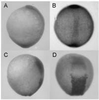 |
Fig. S5 Synergistic effect of zdia2 sMO and profilin I tMO. Embryos were injected with 8 ng zdia2 sMO (A and B) or co-injected with 4 ng zdia2 sMO and 4 ng profilin I tMO (C and D). Embryos were incubated until tail bud stage (10 hpf), fixed and stained with ntl and gsc riboprobe. Photographs were taken for side view (A and C) and dorsal view (B and D) after WISH. |
Into this:
| Gene | Fish | Stage | Anatomy | Assay |
|---|---|---|---|---|
| gsc | wild type (unspecified), MO:diaph2,pfn1 | Bud | prechordal plate | ISH |
| gsc | wild type (unspecified), MO:diaph2 | Bud | prechordal plate | ISH |
| ntla | wild type (unspecified), MO:diaph2,pfn1 | Bud | notochord | ISH |
| ntla | wild type (unspecified), MO:diaph2,pfn1 | Bud | tail bud | ISH |
| ntla | wild type (unspecified), MO:diaph2 | Bud | notochord | ISH |
| ntla | wild type (unspecified), MO:diaph2 | Bud | tail bud | ISH |
| From ZFIN: Figure: Lai et al., 2008, Fig. S5 | | | | |
What defines an expression pattern?
Expression could include a lot of different things, and what it includes depends on the community:
Gene, or Transcript, or Protein, or …
What are we measuring?
Stage
Store single stages, or stage windows?
What do stage windows or adjacent stages mean: throughout window, or we aren’t sure on the stage (high-throughput)
Strain / Genotype
What geneotype did we see this on.
Anatomy
Does “expressed in brain” mean expressed in all, most, or somewhere in
brain?
Assay
ISN, antibody, probe, …
Source
Publication, high-throughput screen, lab, project, …
Genotype
Environment
Pattern
Do you want to keep track of homogeneous, graded, spotty
Not Expressed
Do you keep track of absence? If so, what does it mean? (not detected)
Image
Is an image required or optional?
Strength
What do strengths mean across different experiments?
How does Chado deal with this variety?
Post-composition, which is a very Chadoish way of doing things.
- Embrace a minimal definition of what an expression pattern is. In Chado, all that is required is a name, e.g., SLC21A in GMOD Course Participant kidney after 4 days at NESCent, or just “GMOD0002347”.
- You can also provide a description. If your name is “GMOD0002347”, this may be a good idea
- Details are then hung off that.
FlyBase Example
A specific example from FlyBase:
Here is an example of a simple case of the sort of data that FlyBase curates.
The dpp transcript is expressed in embryonic stage 13-15 in the cephalic segment as reported in a paper by Blackman et al. in 1991.
This would be implemented in the expression module by linking the dpp transcript feature to expression via feature_expression. We would then link the following cvterms to the expression using expression_cvterm:
- embryonic stage 13 where the cvterm_type would be stage and the rank=0
- embryonic stage 14 where the cvterm_type would be stage and the rank=1
- embryonic stage 15 where the cvterm_type would be stage and the rank=1
- cephalic segment where the cvterm_type would be anatomy and the rank=0
- in situ hybridization where the cvterm_type would be assay and the rank=0
Translation
In FlyBase, this would be a single expression record, with 5 Ontology/CV terms attached to it.
- 1 saying what anatomy the expression is for - cephalic segment
- 1 saying that the assay type was in situ hybridization
- 1 each for each of the 3 stages - embryonic stages 13, 14, 15
And
- 1 record saying this expression pattern is for dpp.
- 1 record saying this expression pattern is from Blackman et al. in 1991.
Chado Allows
The Expression module table design allows each expression pattern to have
- 1 name
- 0, 1 or more
- Publications / Sources
- Features
- Images
- Anatomy terms
- Stages
- Assay types
- Any other CV/Ontology term (e.g., detected, not detected)
Two Key Points
- Chado can support whatever your community decides your definition of an expression pattern is.
- However, Chado will not enforce that definition for you.
If you require an expression pattern to have
- 1 name
- 1 publication/source
- 1 Feature
- 1 anatomy term
- 1 stage
- 1 assay type
- 1 detected / not detected flag
- 0, 1 or more images
then you will have to write a script to check that.
Table: expression
| F-Key | Name | Type | Description |
|---|---|---|---|
| expression_id | serial | PRIMARY KEY | |
| uniquename | text | UNIQUE NOT NULL | |
| md5checksum | character(32) | ||
| description | text |
expression Structure
Tables referencing this one via Foreign Key Constraints:
- expression_cvterm, expression_image, expression_pub, expressionprop, feature_expression, wwwuser_expression
Table: expression_cvterm
| F-Key | Name | Type | Description |
|---|---|---|---|
| expression_cvterm_id | serial | PRIMARY KEY | |
| expression | expression_id | integer | UNIQUE#1 NOT NULL |
| cvterm | cvterm_id | integer | UNIQUE#1 NOT NULL |
| rank | integer | NOT NULL | |
| cvterm | cvterm_type_id | integer | UNIQUE#1 NOT NULL |
expression_cvterm Structure
Tables referencing this one via Foreign Key Constraints:
Genotype
Defined in the Chado Genetic Module.
A genotype in Chado is basically a name, with a pile of features associated to it.
This used to mean a set of alleles.
Not sure how strains have been handled
In the era of high-throughput sequencing, this may be much more detailed.
Table: genotype
Genetic context. A genotype is defined by a collection of features, mutations, balancers, deficiencies, haplotype blocks, or engineered constructs.
| F-Key | Name | Type | Description |
|---|---|---|---|
| genotype_id | serial | PRIMARY KEY | |
| name | text | Optional alternative name for a genotype, for display purposes. |
|
| uniquename | text | UNIQUE NOT NULL The unique name for a genotype; typically derived from the features making up the genotype. |
|
| description | character varying(255) |
genotype Structure
Tables referencing this one via Foreign Key Constraints:
Table: feature_genotype
| F-Key | Name | Type | Description |
|---|---|---|---|
| feature_genotype_id | serial | PRIMARY KEY | |
| feature_id | integer | UNIQUE#1 NOT NULL | |
| genotype_id | integer | UNIQUE#1 NOT NULL | |
| chromosome_id | integer | UNIQUE#1 A feature of SO type "chromosome". |
|
| rank | integer | UNIQUE#1 NOT NULL rank can be used for n-ploid organisms or to preserve order. |
|
| cgroup | integer | UNIQUE#1 NOT NULL Spatially distinguishable group. group can be used for distinguishing the chromosomal groups, for example (RNAi products and so on can be treated as different groups, as they do not fall on a particular chromosome). |
|
| cvterm_id | integer | UNIQUE#1 NOT NULL |
feature_genotype Structure
Environment
Also defined in the Chado Genetic Module.
Table: environment
The environmental component of a phenotype description.
| F-Key | Name | Type | Description |
|---|---|---|---|
| environment_id | serial | PRIMARY KEY | |
| uniquename | text | UNIQUE NOT NULL | |
| description | text |
environment Structure
Tables referencing this one via Foreign Key Constraints:
Table: environment_cvterm
| F-Key | Name | Type | Description |
|---|---|---|---|
| environment_cvterm_id | serial | PRIMARY KEY | |
| environment | environment_id | integer | UNIQUE#1 NOT NULL |
| cvterm | cvterm_id | integer | UNIQUE#1 NOT NULL |
environment_cvterm Structure
Phenotype, Natural Diversity and Atlas Support
Phenotypes, natural diversity, and atlas support are all areas of future work in Chado. Chado does have a phenotype module, but it has not aged as well as other modules. Its support for natural diversity is limited to what is implemented in the genotype, environment, and phenotype modules. This is not robust enough to deal with studie that are frequently done in the plant community, and are increasingly done in animal communities as well.
To address this there are several efforts currently underway. The Aniseed project includes 4 dimensional anatomy, expression, and cell fate graphical atlases. Aniseed is currently in the process of reimplementing itself to use Chado. This work is likely to lead to contributions back to GMOD (both in Chado and a web interface) to better support these types of atlases.
Better natural diversity support will be added in the coming year. NESCent has developed a prototype natural diversity Chado module based on the GDPDM, that will added robust support for natural diversity data.
Facts about “Chado Tutorial 2013”
| Has topic | Chado + |