Where p53’s damaging variants fall
TP53 is the gene most often mutated in human cancer, and the mutations are not spread evenly along the protein it encodes. Three independent sources locate the damaging ones: clinical laboratories reporting what they found in patients, a model scoring every substitution that could exist, and a laboratory screen that grew cells carrying thousands of them. This page puts all three on the same p53 alignment, one bar per residue of the human row, over fifteen vertebrates from human to zebrafish, and ends on a link that opens the result.
Prerequisites#
curl,jqandawk- MAFFT and FastTree.
apt install mafft fasttreeon Debian or Ubuntu,brew install mafft fasttreeon macOS, or run the biocontainers with docker:quay.io/biocontainers/mafft:7.525--h031d066_1andquay.io/biocontainers/fasttree:2.1.11--h031d066_4. The build script takes either. - nothing to read along: every figure below links to the live view it captured
Where the data comes from#
Sequences from NCBI RefSeq, the clinical classifications from ClinVar, the predictions from AlphaMissense as the AlphaFold entry publishes them, and one saturation screen from MaveDB.
- the 660 vertebrate orthologs NCBI lists for TP53, GeneID 7157, the source of the accession list below: https://api.ncbi.nlm.nih.gov/datasets/v2alpha/gene/id/7157/orthologs?taxon_filter=vertebrates
- one protein per accession, all fifteen in one request: https://eutils.ncbi.nlm.nih.gov/entrez/eutils/efetch.fcgi?db=protein&id=NP_000537.3&rettype=fasta&retmode=text
- ClinVar’s TP53 missense records, searched and then summarized: https://eutils.ncbi.nlm.nih.gov/entrez/eutils/esearch.fcgi?db=clinvar&retmax=5000&term=TP53%5Bgene%5D+AND+%22missense+variant%22%5Bmolecular+consequence%5D
- the AlphaFold entry for P04637, which names its AlphaMissense file: https://alphafold.ebi.ac.uk/api/prediction/P04637
- that file, 7,467 substitutions with a pathogenicity score each: https://alphafold.ebi.ac.uk/files/AF-P04637-F1-aa-substitutions.csv
- the Giacomelli 2018 screen, scores for 8,274 variants, CC0: https://api.mavedb.org/api/v1/score-sets/urn:mavedb:00000068-a-1/scores
- the domain boundaries the bands draw, as UniProt annotates them: https://rest.uniprot.org/uniprotkb/P04637.json?fields=ft_domain,ft_region
- the alignment the commands below write, hosted so the figures can link to it: https://gmod.org/JBrowseMSA/demo/data/p53/p53-vertebrates.afa
- its tree: https://gmod.org/JBrowseMSA/demo/data/p53/p53-vertebrates.nh
- the three tracks, as the viewer takes them: https://gmod.org/JBrowseMSA/demo/data/p53/p53-layers.json
1. Name the rows#
NCBI’s ortholog set for TP53 is large, so this step chooses rows from it:
curl -s 'https://api.ncbi.nlm.nih.gov/datasets/v2alpha/gene/id/7157/orthologs?taxon_filter=vertebrates&page_size=1000' |
  jq -r '.reports[].gene | [.taxname, .common_name, .gene_id] | @tsv'
The query returns 660 species. The list below takes fifteen, spread from human
to zebrafish, with one RefSeq protein accession each and the label the viewer
draws down the side. Human is NP_000537.3, the product of NM_000546. ClinVar
names its variants on the same transcript, so residue 248 is the same residue in
every file on this page.
NP_000537.3	Human
XP_045231359.1	Macaque
XP_027375188.1	Cow
XP_047612858.1	Pig
NP_001189334.1	Horse
XP_025284307.1	Dog
XP_010594888.1	Elephant
XP_030101782.1	Mouse
NP_112251.2	Rat
XP_056673571.1	Opossum
NP_990595.1	Chicken
XP_065426476.1	Turtle
XP_062840611.1	Anole
NP_001001903.1	Frog
XP_073805887.1	Zebrafish
Save that as accessions.tsv, tab separated.
2. Fetch the sequences#
One request takes the whole list, and an awk pass renames each record from its
accession to its label:
IDS=$(cut -f1 accessions.tsv | paste -sd,)
curl -sf "https://eutils.ncbi.nlm.nih.gov/entrez/eutils/efetch.fcgi?db=protein&id=$IDS&rettype=fasta&retmode=text" \
  > p53-refseq.fa

# every layer below names a row by the label the viewer draws
awk 'NR == FNR {split($0, row, "\t"); label[row[1]] = row[2]; next}
  /^>/ {split($0, field, " "); print ">" label[substr(field[1], 2)]; next}
  NF {print}' accessions.tsv p53-refseq.fa > p53.fasta
Check the lengths before aligning them:
awk '/^>/ {if (name) print name, n; name = $0; n = 0; next} {n += length($0)}
  END {print name, n}' p53.fasta
>Human 393
>Macaque 393
>Cow 386
>Pig 386
>Horse 381
>Dog 381
>Elephant 390
>Mouse 390
>Rat 391
>Opossum 361
>Chicken 367
>Turtle 409
>Anole 395
>Frog 362
>Zebrafish 374The fifteen records run from 361 to 409 residues, and every one is full length. A truncated model or a stray isoform would show up in this list as an outlying length.
3. Align them and infer a tree#
# --anysymbol accepts a record with an X or a U in it
mafft --auto --anysymbol p53.fasta > p53.afa

# -lg is the amino-acid substitution model; FastTree reads the alignment and
# writes Newick with a support value on each internal node
FastTree -lg -quiet p53.afa > p53.nh
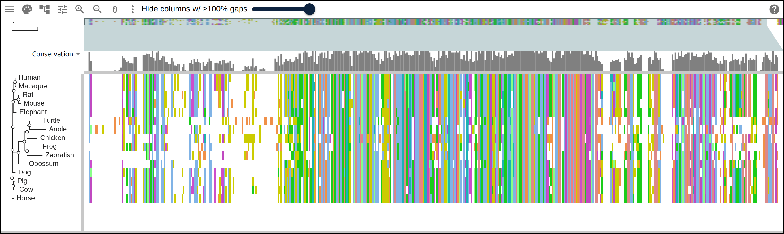
The alignment has 478 columns against a longest input of 409, so MAFFT opened 69 columns of insertions, most of them in the N terminus. The tree puts the two rodents together at support 1.000 and human with macaque at 0.997. The deep splits come out at 0.295 and 0.310, too low to resolve from 478 columns, so the tree orders the rows for reading and its deep topology is unsupported.
4. Ask ClinVar which residues patients are diagnosed on#
ClinVar holds variants that laboratories submitted with a clinical classification. The search takes the gene and the consequence, and the script filters the classification from the records themselves, because an esearch term matching “pathogenic” also pulls in “Conflicting classifications of pathogenicity”:
EUTILS=https://eutils.ncbi.nlm.nih.gov/entrez/eutils
TERM='TP53[gene] AND "missense variant"[molecular consequence]'
curl -sf "$EUTILS/esearch.fcgi?db=clinvar&retmode=json&retmax=5000&term=$(
  jq -rn --arg t "$TERM" '$t | @uri'
)" | jq -r '.esearchresult.idlist[]' > clinvar.ids

# esummary takes 200 ids at a time. Keep only what the submitters classify as
# pathogenic, and take the variant name, which carries the protein change
split -l 200 clinvar.ids clinvar.batch.
for batch in clinvar.batch.*; do
  curl -sf "$EUTILS/esummary.fcgi?db=clinvar&retmode=json&id=$(paste -sd, "$batch")" |
    jq -r '.result | del(.uids) | .[]
      | select(.germline_classification.description
        | IN("Pathogenic", "Likely pathogenic", "Pathogenic/Likely pathogenic"))
      | .variation_set[].variation_name' >> clinvar.changes
  # NCBI asks unauthenticated callers to stay under three requests a second
  sleep 0.4
done
The search returns 1,519 missense records, and 253 of them pass that filter. The
count per residue comes from reading p.Arg248Gln out of
NM_000546.6(TP53):c.743G>A (p.Arg248Gln):
grep '^NM_000546' clinvar.changes |
  grep -oE '\(p\.[A-Z][a-z]{2}[0-9]+[A-Z][a-z]{2}\)' |
  grep -v 'Ter)$' |
  grep -oE '[0-9]+' |
  awk -v n=393 '{count[$1]++}
    END {for (i = 1; i <= n; i++) printf "%s%d", (i > 1 ? "," : ""), count[i]}'
grep -v 'Ter)$' drops the nonsense changes. A stop truncates everything
downstream of it instead of exchanging one residue, so the per-residue count of
substitutions leaves it out.
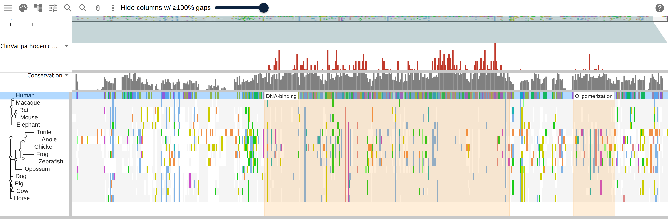
The 253 variants land on 104 of the 393 residues, 94% of them inside the DNA-binding domain, and the deepest single residue is 281 with 8 of them.
5. Ask AlphaMissense what it predicts#
AlphaMissense scores every substitution a protein could have, whether or not anyone has seen it. The AlphaFold entry for an accession names the file:
AM_URL=$(curl -sf https://alphafold.ebi.ac.uk/api/prediction/P04637 |
  jq -r '.[0].amAnnotationsUrl')
curl -sf "$AM_URL" -o alphamissense.csv
The file has 7,467 rows, 19 substitutions at each of 393 residues, each scored
from 0 to 1. The script takes one mean per residue, reading the position out of
the M1A in the first column:
tail -n +2 alphamissense.csv |
  awk -F, -v n=393 '{
    pos = substr($1, 2, length($1) - 2)
    sum[pos] += $2
    seen[pos]++
  }
  END {for (i = 1; i <= n; i++)
    printf "%s%.2f", (i > 1 ? "," : ""), (seen[i] ? sum[i] / seen[i] : 0)}'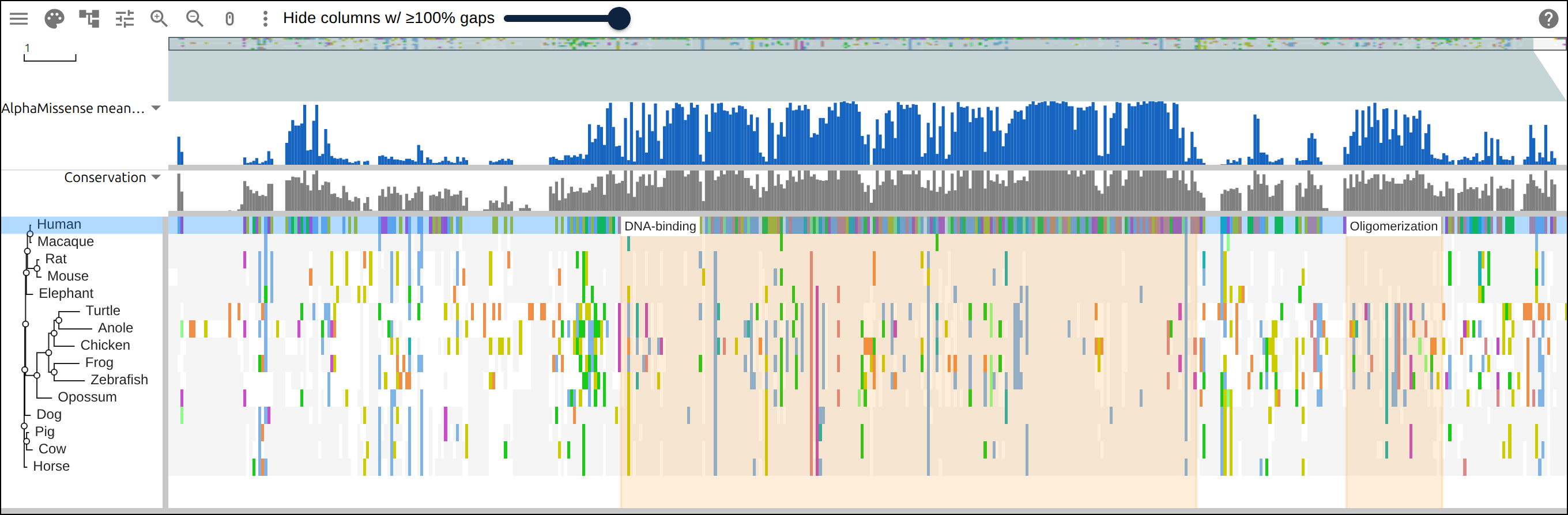
6. Ask a saturation screen what it measured#
Giacomelli and colleagues put a library of p53 variants into A549 cells that keep a wild-type copy of the gene, selected with nutlin-3, and sequenced what grew. A variant that enriches under that selection has knocked out p53’s function in the presence of the wild-type protein. MaveDB serves the scores as CC0:
curl -sfL https://api.mavedb.org/api/v1/score-sets/urn:mavedb:00000068-a-1/scores \
  -o mavedb.csv

# the score column against the protein change; p.Met384= is synonymous and
# p.Arg248Ter is a stop, and neither is one residue exchanged for another
tail -n +2 mavedb.csv |
  awk -F, -v n=393 '$4 ~ /^p\.[A-Z][a-z][a-z][0-9]+[A-Z][a-z][a-z]$/ &&
    $4 !~ /Ter$/ && $5 != "NA" {
    match($4, /[0-9]+/)
    pos = substr($4, RSTART, RLENGTH)
    sum[pos] += $5
    seen[pos]++
  }
  END {for (i = 1; i <= n; i++) {
    mean = seen[i] ? sum[i] / seen[i] : 0
    printf "%s%.2f", (i > 1 ? "," : ""), (mean > 0 ? mean : 0)
  }}'
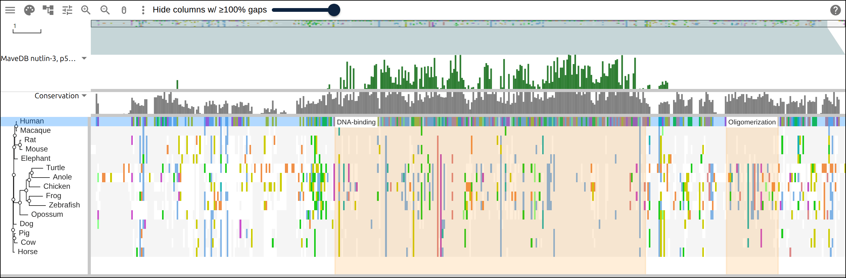
The file holds 8,274 variants, 7,487 of them missense with a score. The screen
used a P72R background, so its residue 72 is an arginine where the RefSeq
protein this page aligns has a proline. A bar track clamps at zero, so
(mean > 0 ? mean : 0) writes zero for a negative mean. About half the residues
come out at or below zero and draw nothing.
7. Put the three on one set of columns#
Each track is a columnTracks entry naming the row its values index, so the
viewer places values in the human protein’s residue numbering on the alignment
columns fifteen species share:
jq -rj --arg msa data/p53/p53-vertebrates.afa \
  --arg tree data/p53/p53-vertebrates.nh '
  {
    msaview: {
      type: "MsaView",
      relativeTo: "Human",
      colorSchemeName: "clustalx_protein_dynamic",
      msaFilehandle: {uri: $msa},
      treeFilehandle: {uri: $tree},
      highlights: .highlights,
      columnTracks: .columnTracks
    }
  } | @uri' p53-layers.json
@uri is the last step because the whole snapshot travels in the link. The
server stops serving a request line past 8,192 characters, and this one is 7,820
with three tracks of 393 values in it. AlphaMissense goes in as a percent
against max: 100 to save room, since 0.87, costs five characters and 87,
costs three.
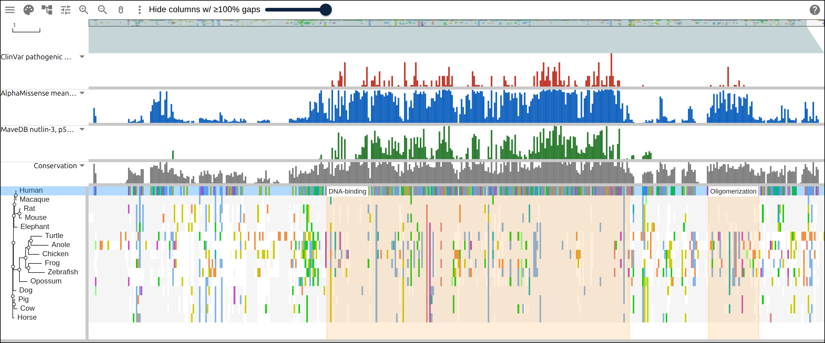
Averaged over the regions UniProt annotates:
| Region | ClinVar | AlphaMissense | MaveDB |
|---|---|---|---|
| Transactivation 1-44 | 0.00 | 0.31 | 0.02 |
| Proline-rich 50-96 | 0.00 | 0.22 | 0.00 |
| DNA-binding 102-292 | 1.25 | 0.75 | 0.79 |
| Oligomerization 325-356 | 0.41 | 0.59 | 0.00 |
8. The hotspot columns#
The six residues cancer genomes mutate most often are R175, G245, R248, R249, R273 and R282, all of them inside the DNA-binding domain. At base resolution the alignment shows which residue each vertebrate carries there:
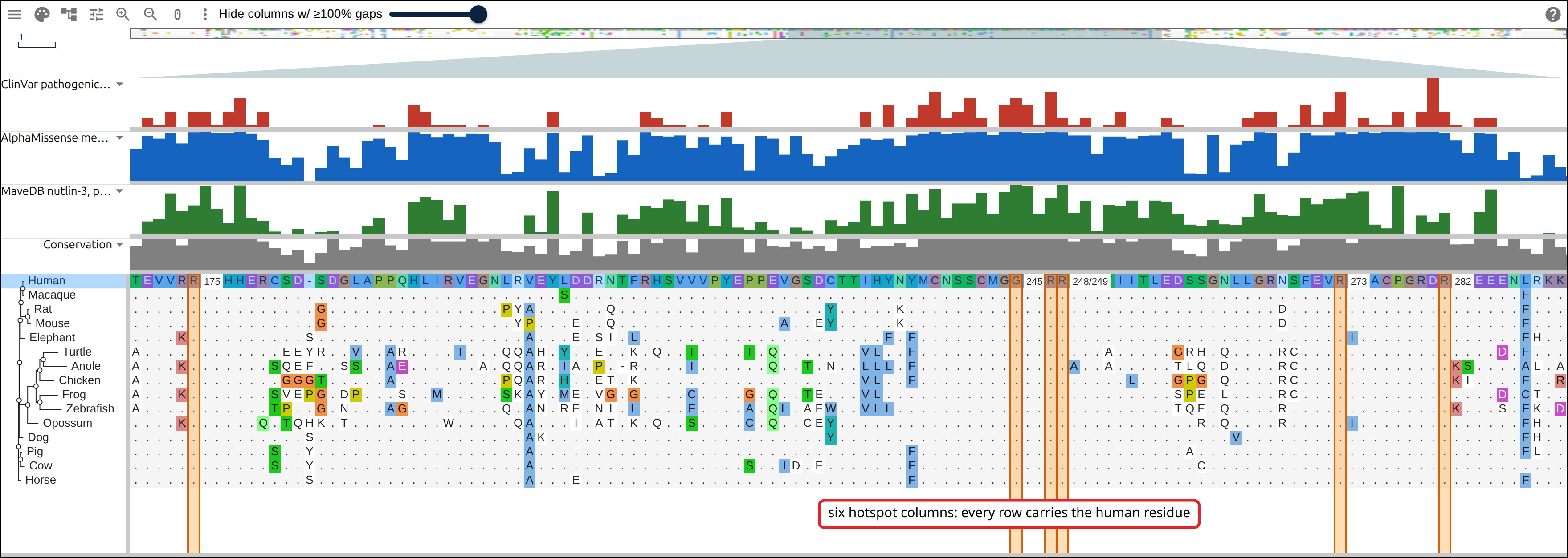
Counting the rows that carry the human residue in each of those columns, against three residues from the N terminus:
| Residue | Human | Rows with it | Rows gapped |
|---|---|---|---|
| R175 | R | 15/15 | 0 |
| G245 | G | 15/15 | 0 |
| R248 | R | 15/15 | 0 |
| R249 | R | 15/15 | 0 |
| R273 | R | 15/15 | 0 |
| R282 | R | 15/15 | 0 |
| P47 | P | 6/15 | 0 |
| P72 | P | 4/15 | 7 |
| P89 | P | 4/15 | 0 |
Zebrafish and human last shared an ancestor more than 400 million years ago and both still carry an arginine at 248.
9. The control, at the other end of the protein#
The first hundred residues are the transactivation domain and the proline-rich region, which UniProt annotates as disordered and where the alignment is mostly letters and gaps. The figure uses the same zoom as the hotspot figure:
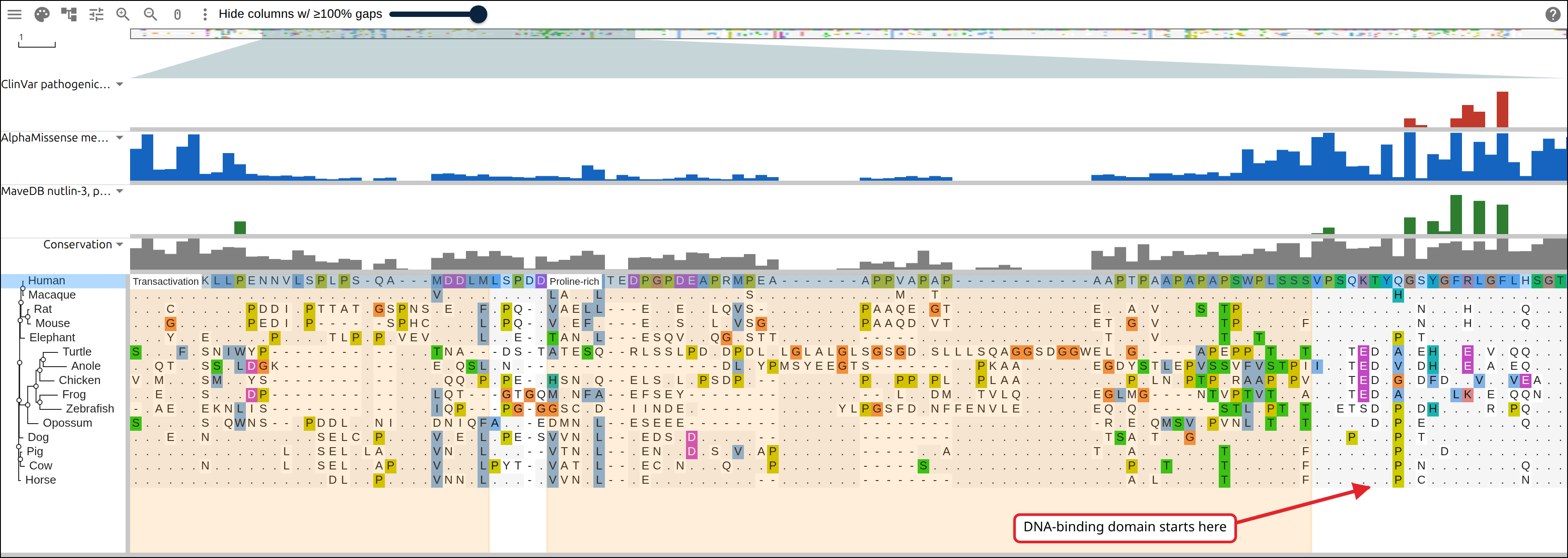
ClinVar has no pathogenic missense variant anywhere in either region. The screen averages 0.02 and 0.00 over them. AlphaMissense scores them at 0.31 and 0.22, against 0.75 for the DNA-binding domain.
10. The oligomerization domain#
The oligomerization domain is the other structured part of p53, the helix that makes the tetramer. AlphaMissense scores it at 0.59 against 0.75 for the DNA-binding domain, ClinVar has 13 pathogenic missense variants across its 32 residues, and the screen comes out at zero on all 32, because every raw mean there is zero or negative:
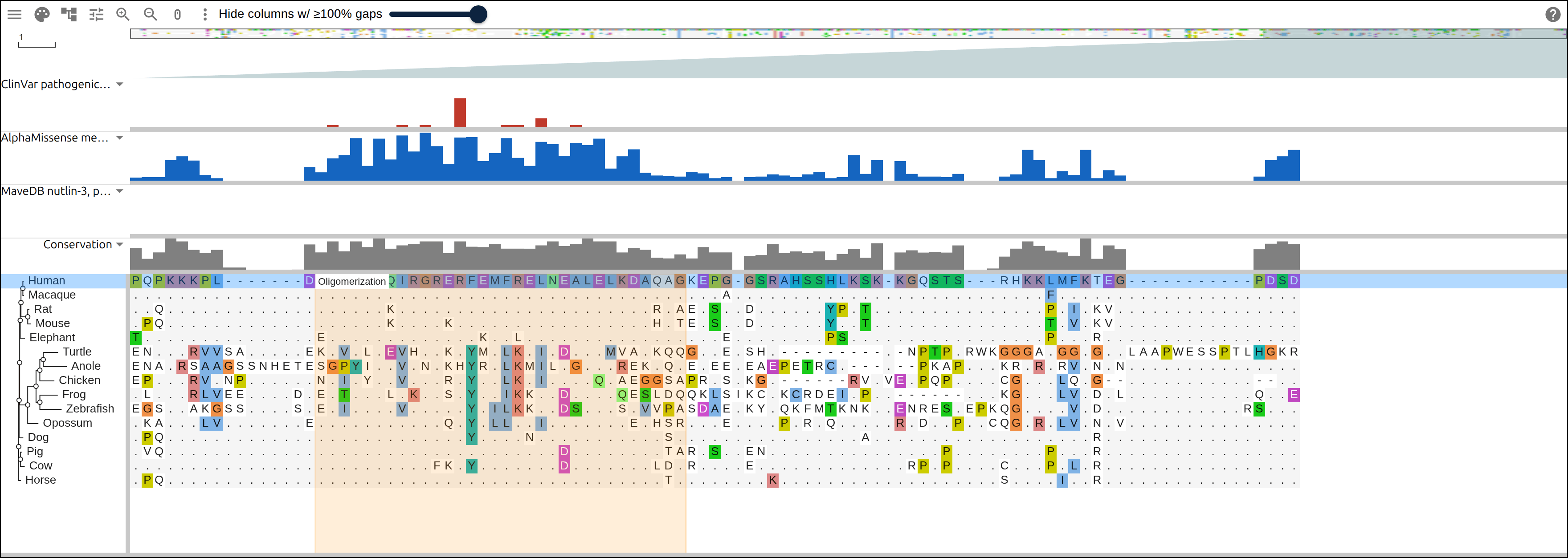
The screen selected for variants that disable p53 while a wild-type copy of the protein is present in the same cell, which is a narrower question than whether the variant breaks the protein.
11. Check a residue against the files#
Every bar on this page is an aggregate of a source file, and a grep recovers it. R248 against P47:
grep 'p.Arg248' clinvar.changes                          # 6 variants
grep -E '^R248' alphamissense.csv |
  awk -F, '{s += $2; n++} END {printf "%.2f over %d\n", s / n, n}'   # 1.00 over 19
grep -E 'p\.Arg248[A-Z]' mavedb.csv | grep -v Ter |
  awk -F, '{s += $5; n++} END {printf "%.2f over %d\n", s / n, n}'   # 1.50 over 19
The same three at P47 return 0 variants, 0.15 over 19, and a negative MaveDB mean. The build script writes a negative mean as 0, since the track clamps at zero, so the residue draws nothing there.
The six ClinVar records at 248 are c.742C>T and c.741_742delinsTT, both
p.Arg248Trp, plus Gly, Pro, Leu and Gln. A count here is variants on record,
which is not patients: two rows reaching the same tryptophan by different
nucleotide changes are two records.
Reproduce it end to end#
curl -O https://raw.githubusercontent.com/GMOD/JBrowseMSA/main/docs/tutorials/scripts/build_p53_variant_effects.sh
bash build_p53_variant_effects.sh out/
The script writes the accession list, fetches and aligns the sequences, builds
the three tracks, prints every table above, and leaves the link in
out/p53-link.url. Prerequisites lists the tools it needs,
and it runs the biocontainers when MAFFT and FastTree are not on PATH. ClinVar
is updated weekly, so its counts drift between runs where the alignment and the
two files with a fixed release do not.
Here is what that link opens, against the hosted copy of this alignment.
See also#
References#
- Landrum MJ, et al. ClinVar: improving access to variant interpretations and supporting evidence. Nucleic Acids Research 46:D1062-D1067 (2018).
- Cheng J, et al. Accurate proteome-wide missense variant effect prediction with AlphaMissense. Science 381:eadg7492 (2023).
- Varadi M, et al. AlphaFold Protein Structure Database in 2024. Nucleic Acids Research 52:D368-D375 (2024), which serves the AlphaMissense file above.
- Giacomelli AO, et al. Mutational processes shape the landscape of TP53
mutations in human cancer. Nature Genetics 50:1381-1387 (2018), the screen
behind
urn:mavedb:00000068-a-1. - Esposito D, et al. MaveDB: an open-source platform to distribute and interpret data from multiplexed assays of variant effect. Genome Biology 20:223 (2019).
- Katoh K, Standley DM. MAFFT multiple sequence alignment software version 7. Molecular Biology and Evolution 30:772-780 (2013).
- Price MN, Dehal PS, Arkin AP. FastTree 2, approximately maximum-likelihood trees for large alignments. PLoS ONE 5:e9490 (2010).