Eight mitochondrial genomes and the genes on them
A mammal mitochondrial genome is about 16.5 kb and carries 37 genes: 13 protein subunits of the respiratory chain, 2 rRNAs and 22 tRNAs, in an order shared across the vertebrates. This page takes eight of them from RefSeq, aligns them, and derives one GFF that names each gene, gives it a strand, and records the respiratory complex its product belongs to. The viewer draws each gene as an arrow in the alignment’s columns, filled by complex and labeled by name.
Prerequisites#
curl- ClustalW,
apt install clustalwon Debian or Ubuntu,brew install clustal-won macOS. ClustalW both aligns and infers a tree, so this page needs no other aligner. - Python 3, for the step that reshapes RefSeq’s GFF3
Every figure below links to the live view it captured.
Where the data comes from#
Eight mammal mitochondrial genomes as RefSeq holds them, with RefSeq’s own annotation of each.
- one genome per accession: https://eutils.ncbi.nlm.nih.gov/entrez/eutils/efetch.fcgi?db=nuccore&id=NC_012920.1&rettype=fasta&retmode=text
- its annotation as GFF3: https://www.ncbi.nlm.nih.gov/sviewer/viewer.fcgi?id=NC_012920.1&report=gff3&retmode=text
- the eight genomes before alignment, right-padded to one width so the viewer opens them: https://gmod.org/JBrowseMSA/demo/data/mitogenome/mito-unaligned.afa
- the alignment the commands below write, hosted so the figures can link to it: https://gmod.org/JBrowseMSA/demo/data/mitogenome/mito.afa
- its tree: https://gmod.org/JBrowseMSA/demo/data/mitogenome/mito.nwk
- its genes: https://gmod.org/JBrowseMSA/demo/data/mitogenome/mito-genes.gff
Both endpoints serve one accession per request, so the eight genomes take eight requests to each.
The genomes#
Write one RefSeq accession per line, followed by the label you want down the side of the viewer. The label becomes the FASTA defline, the tree tip, and column 1 of the gene GFF.
NC_012920.1	Human
NC_001643.1	Chimp
NC_005089.1	Mouse
NC_001665.2	Rat
NC_002008.4	Dog
NC_006853.1	Cow
NC_001640.1	Horse
NC_000891.1	Platypus
Save that as mito-rows.tsv. The separator is a tab.
Platypus is the outgroup here, and it keeps the gene order the other seven have. Marsupial mitogenomes carry the five tRNAs between ND2 and COX1 in another order, so an opossum row would put those five arrows somewhere else along its own row.
1. Fetch the genomes and their annotations#
while IFS=$'\t' read -r accession label; do
  curl -sf "https://eutils.ncbi.nlm.nih.gov/entrez/eutils/efetch.fcgi?db=nuccore&id=$accession&rettype=fasta&retmode=text" \
    -o "raw/$accession.fa"
  curl -sf "https://www.ncbi.nlm.nih.gov/sviewer/viewer.fcgi?id=$accession&report=gff3&retmode=text" \
    -o "raw/$accession.gff"
done < mito-rows.tsv
Count what came back before aligning it:
  Human        NC_012920.1  16569 bp  37 genes
  Chimp        NC_001643.1  16554 bp  37 genes
  Mouse        NC_005089.1  16299 bp  37 genes
  Rat          NC_001665.2  16313 bp  37 genes
  Dog          NC_002008.4  16727 bp  37 genes
  Cow          NC_006853.1  16338 bp  37 genes
  Horse        NC_001640.1  16660 bp  37 genes
  Platypus     NC_000891.1  17019 bp  37 genes
All eight have 37 genes. The lengths run 720 bp apart, from 16,299 in Mouse to 17,019 in Platypus, and most of that difference is in the control region.
The viewer opens the genomes as they come, once every row is the same length. Right-pad the shorter ones to 17,019 and the eight load as a block.

2. Align them and build a tree#
clustalw -INFILE=mito.fasta -ALIGN -TYPE=DNA \
  -OUTPUT=FASTA -OUTFILE=mito.afa

# -TREE reads an existing alignment and writes neighbor-joining Newick;
# ClustalW wraps it across lines, and the viewer wants one string
clustalw -INFILE=mito.afa -TREE -TYPE=DNA -OUTPUTTREE=phylip
tr -d '[:space:]' < mito.ph > mito.nwk
Eight whole mitogenomes take about three minutes on a laptop. ClustalW reports
Alignment Score 2191242 and 17,966 columns, 947 more than the longest input,
which is the room it made for insertions.
(((((Mouse:0.08782,Rat:0.08393):0.04922,Platypus:0.17510):0.00685,
(Human:0.04074,Chimp:0.04555):0.10155):0.01849,Cow:0.09959):0.00282,
Dog:0.11305,Horse:0.09847);
Platypus has the longest branch in the tree, 0.17510 where the rest run 0.04 to 0.11, and neighbor joining draws it next to the rodents. The tree here orders the rows.

3. Derive the gene GFF#
RefSeq’s GFF3 has a gene line, an RNA or CDS line and an exon line per gene,
in that genome’s coordinates and under that genome’s accession. The viewer wants
one line per gene, under the row label, carrying the fields the marks read: the
name, the strand, an attribute naming the respiratory complex, and a color= on
the one feature that carries its own color.
The 13 protein genes are ND1 to ND6 and ND4L in complex I, CYTB in
complex III, COX1 to COX3 in complex IV, and ATP6 with ATP8 in complex
V:
# the four complexes mtDNA encodes subunits of. Complex II is nuclear
COMPLEX = {'ND1': 'I', 'ND2': 'I', 'ND3': 'I', 'ND4': 'I', 'ND4L': 'I',
           'ND5': 'I', 'ND6': 'I', 'CYTB': 'III', 'COX1': 'IV', 'COX2': 'IV',
'COX3': 'IV', 'ATP6': 'V', 'ATP8': 'V'}ND1, COX1, CYTB and the other eleven are the gene Name in every RefSeq
mitogenome. The tRNA and rRNA genes carry a locus tag in five of the eight, so
the script names a tRNA from the product of its child feature (tRNA-Phe) and
the two rRNAs by their order along the genome (RNR1, RNR2). Each gene then
writes one line:
print(f'{label}\tRefSeq\tgene\t{start}\t{end}\t.\t{strand}\t.'
      f'\tName={name};complex={klass}', file=out)
The control region is what follows the last gene, tRNA-Pro. RefSeq annotates it
as D_loop in six of the eight genomes, so the script derives it the same way
for all eight, and gives it a color of its own:
print(f'{label}\tRefSeq\tD_loop\t{last + 1}\t{length}\t.\t.\t.'
      f'\tName=control region;color=255,205,0', file=out)
The first lines of the result:
##gff-version 3
Human	RefSeq	gene	577	647	.	+	.	Name=tRNA-Phe;complex=tRNA
Human	RefSeq	gene	648	1601	.	+	.	Name=RNR1;complex=rRNA
Human	RefSeq	gene	1602	1670	.	+	.	Name=tRNA-Val;complex=tRNA
Human	RefSeq	gene	1671	3229	.	+	.	Name=RNR2;complex=rRNA
Human	RefSeq	gene	3230	3304	.	+	.	Name=tRNA-Leu-1;complex=tRNA
Human	RefSeq	gene	3307	4262	.	+	.	Name=ND1;complex=I
and what it holds:
  I: 56
  III: 8
  IV: 24
  V: 16
  rRNA: 16
  tRNA: 176
  control region: 8
304 features over eight rows: 37 genes and one control region per genome. Positions are 1-based in each genome’s own sequence, and the viewer projects them through that row’s gaps.

4. Fill the arrows by respiratory complex#
featureFill names the field the overlay colors each span by, and a map scale
gives each value of that field a color. Six values appear in the file, so the
map has six entries:
"encodings": [
  {
    "channel": "featureFill",
    "field": "complex",
    "scale": {
      "map": {
        "I": "#4e79a7",
        "III": "#59a14f",
        "IV": "#e15759",
        "V": "#b07aa1",
        "rRNA": "#f28e2b",
        "tRNA": "#bab0ac"
      }
    }
  },
  { "channel": "featureLabel", "field": "Name" }
]
The legend has no entry for complex II. All four of its subunits are encoded in
the nucleus, so no line in the file carries complex=II, and a map entry for
a value the data never takes would draw nothing.
5. Read the gene names off the arrows#
featureLabel names the field drawn inside each span. The viewer draws the
label wherever the text fits inside the arrow’s body, so how many labels appear
follows the column width.
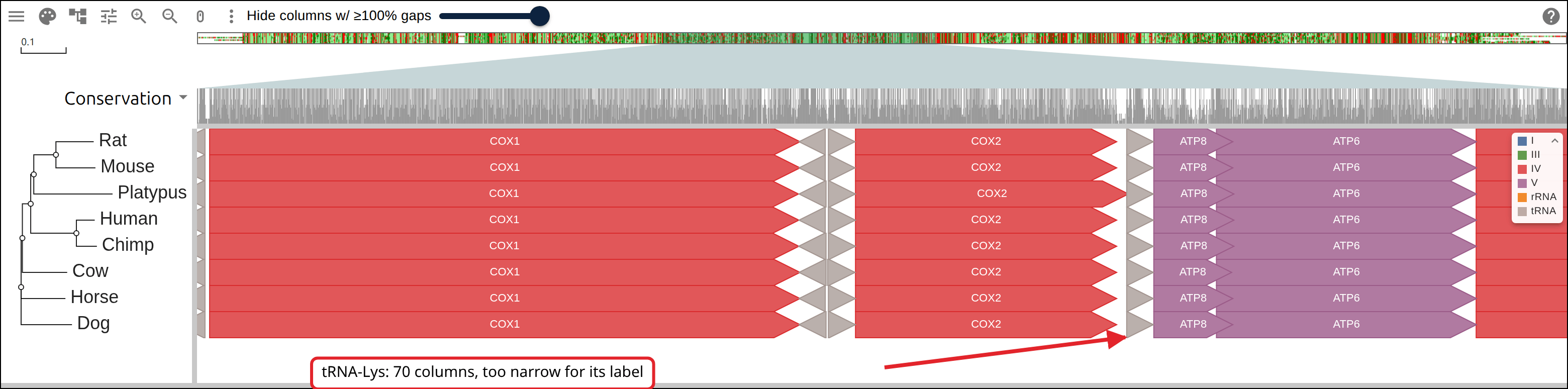
The label is a data channel, so it draws whether or not the residue letters do. At 0.38 pixels per column there are no letters on screen at all.
6. Where each gene lands#
Each row’s positions are its own, and the overlay projects them through that row’s gaps before drawing. COX1 starts at a different base in all eight genomes and at one column in all eight:
COX1:
  Human     bp   5904 -> columns 6134-7676
  Chimp     bp   5321 -> columns 6134-7676
  Mouse     bp   5328 -> columns 6134-7679
  Rat       bp   5323 -> columns 6134-7679
  Dog       bp   5349 -> columns 6134-7679
  Cow       bp   5687 -> columns 6134-7679
  Horse     bp   5362 -> columns 6134-7679
  Platypus  bp   5389 -> columns 6134-7675
Human 5,904 and Chimp 5,321 are 583 bases apart, and both start in column 6,134. The same projection for all 15 named genes, as the spread between the leftmost row and the rightmost:
feature          start spread end spread
RNR1                        1          0
RNR2                        0          0
ND1                        88          4
ND2                         0          2
COX1                        0          4
COX2                        0         31
ATP8                        0          6
ATP6                        0          0
COX3                        0          3
ND3                         0          6
ND4L                        4          0
ND4                         0          0
ND5                         9         26
ND6                        13          0
CYTB                        0          5
control region             10       1091
22 tRNAs: worst start-column spread 5
Ten of the 15 start in one column in every row. ND1 has the widest spread at 88: Mouse and Rat put its first base in column 3,414 and its second in column 3,503, where the other six start in column 3,502.
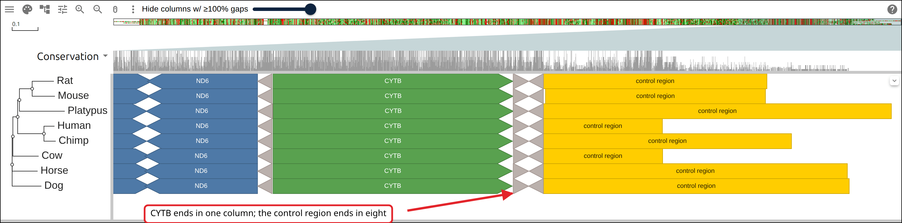
The control region is the last line of that table. Its end spread is 1,091 columns where no gene’s exceeds 31, and the eight right edges land on eight different columns: Human at 16,875, Cow at 16,876, Mouse at 17,366, Rat at 17,373, Chimp at 17,490, Horse at 17,756, Dog at 17,765 and Platypus at 17,966.
7. Share the view#
The three files go in the alignment, tree and annotation slots of the import form, as local files or as URLs. To put the whole view in a link, name the URLs and carry the encodings in the snapshot:
{
  "msaview": {
    "type": "MsaView",
    "colWidth": 0.065,
    "msaFilehandle": { "uri": "https://example.org/mito.afa" },
    "treeFilehandle": { "uri": "https://example.org/mito.nwk" },
    "gffFilehandle": { "uri": "https://example.org/mito-genes.gff" },
    "encodings": [
      {
        "channel": "featureFill",
        "field": "complex",
        "scale": {
          "map": {
            "I": "#4e79a7",
            "III": "#59a14f",
            "IV": "#e15759",
            "V": "#b07aa1",
            "rRNA": "#f28e2b",
            "tRNA": "#bab0ac"
          }
        }
      },
      { "channel": "featureLabel", "field": "Name" }
    ],
    "highlights": [{ "start": 6134, "end": 7679, "label": "COX1" }]
  }
}
URL-encode that and append it to the app as #data=. The link carries the
addresses of the files, so it works at any size. highlights takes 1-based
inclusive columns, and the COX1 span above is the one the projection printed.

The band covers the columns the projection put COX1 in. RefSeq’s GFF3 gives its position in the human genome:
grep -P '\tgene\t' raw/NC_012920.1.gff | grep 'Name=COX1'NC_012920.1 RefSeq gene 5904 7445 . + . ID=gene-COX1;Dbxref=GeneID:4512,HGNC:HGNC:7419,MIM:516030;Name=COX1;gbkey=Gene;gene=COX1;gene_biotype=protein_coding;gene_synonym=COI,MTCO1grep -P '^Human\t' mito-genes.gff | grep 'Name=COX1;'Human RefSeq gene 5904 7445 . + . Name=COX1;complex=IV5904 to 7445 on the plus strand in both files.
Reproduce it end to end#
curl -O https://raw.githubusercontent.com/GMOD/JBrowseMSA/main/docs/tutorials/scripts/build_mitogenome_genes.sh
bash build_mitogenome_genes.sh
With no arguments the script writes the accession list above and builds the files beside it, printing every number this page quotes. Point it at your own list of RefSeq mitochondrial genomes to do the same for another set:
bash build_mitogenome_genes.sh my-rows.tsv out/See also#
References#
- Anderson S, et al. Sequence and organization of the human mitochondrial genome. Nature 290:457-465.
- Boore JL. Animal mitochondrial genomes. Nucleic Acids Research 27:1767-1780.
- O’Leary NA, et al. Reference sequence (RefSeq) database at NCBI. Nucleic Acids Research 44:D733-D745.
- Larkin MA, et al. Clustal W and Clustal X version 2.0. Bioinformatics 23:2947-2948.