GMOD
Introduction to Chado
Contents
- 1 What’s a chado?
- 2 Chado - the way of tea
- 3 What Documentation Exists for chado?
- 4 A Modular Schema
- 5 The Sequence Module and Features
- 6 Feature Graphs
- 7 Feature Graph Transformations
- 8 Representing Graphs in a Relational Database
- 9 Representing Ontology Graphs in Chado
- 10 Representing Feature Graphs in Chado
- 11 Querying Graphs
- 12 Using views to simplify queries
- 13 Extensible Attributes
- 14 Localising Features in Sequence Coordinates
- 15 Interbase Coordinates
- 16 Basic example - with locations
- 17 Locations can be nested
- 18 Computational analysis: Predictions
- 19 Computational analysis: Similarity results
- 20 Computational analysis: Multiple alignments
- 21 Variation features
- 22 Bioperl and chado mapping
- 23 Acknowledgements
- 24 About this Page
What’s a chado?
- At first, a database for FlyBase: incredibly interesting dataset
- A database for very deep curation
- An integrated database
- A database that is generic enough to use for any organism
Chado - the way of tea
Why the reference to tea? According to ancient GMOD lore, legend has it that creators Chris Mungall and Dave Emmert were drinking tea in a tea house when they developed the first design that eventually became Chado.
What Documentation Exists for chado?
This Wiki is currently the best source of documentation for Chado. Here are more useful pages in the Wiki:
A Modular Schema
Chado Module List
- Audit - for database audit trails
- Companalysis - for data from computational analysis
- Contact - for people, groups, and organizations
- Controlled Vocabulary (cv) - for controlled vocabularies and ontologies
- Expression - for summaries of RNA and protein expresssion
- General - for identifiers
- Genetic - for genetic data and genotypes
- Library - for descriptions of molecular libraries
- Mage - for microarray data
- Map - for maps without sequence
- Natural Diversity (ND) - for multiple experiments, such as phenotyping and genotyping
- Organism - for taxonomic data
- Phenotype - for phenotypic data
- Phylogeny - for organisms and phylogenetic trees
- Publication (pub) - for publications and references
- Sequence - for sequences and sequence features
- Stock - for specimens and biological collections
- WWW -
There are dependencies between the modules.
This page is focused on the sequence module; we will also discuss parts of the cv module as ontologies are crucial to how chado represents all data.
The actual chado tables themselves are not discussed in attribute-by-attribute detail; this can be browsed by checking out the Chado Manual.
One of the main strengths of chado is that it brings the sequence and genetics views of the world together.
Let’s look at the chado conceptualisation of the world before diving in to the schema design.
The Sequence Module and Features
Definition
- A feature is a thingy
- A feature is a potentially localisable
- A feature is further defined by an ontology
Feature Types: an Ontology
One way of representing ontologies is through a graph model, with nodes representing concepts and edges representing relationship types between the concepts.
Simplified Sequence Ontology
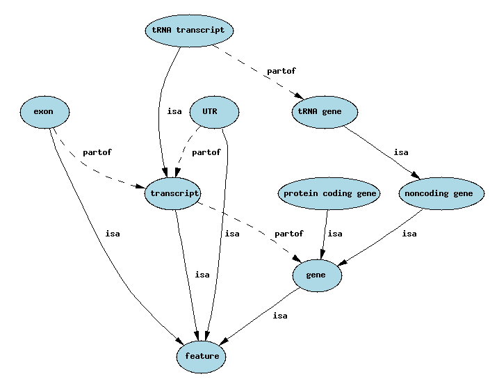
is_a: subtypes, specialisation/generalization
part_of: compositional
Some other feature types
- HSP
- protein domain
- chromosome arm
- contig
- scaffold
- regulatory region
- variation features: insertions, deletions, SNPs
Feature Graphs
| Problem/Question: The compositional relationships are a subset of the relationships from gene to CDS in SO. How does one decide where to simplify the graph? |
The nodes in the graph represent instances of features - the arcs in these cases represent compositional relationships (although other relationship types are possible). Feature graphs do not represent positional or spatial relationships - we will get to that later. For more on representing genes also see Chado Best Practices.
Basic Central Dogma Example
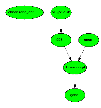
One gene, one transcript, one exon, one protein
Alternate Splicing
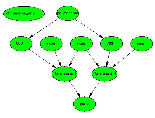
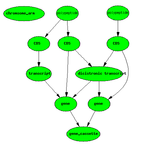
Dicistronic Gene
A dicistronic gene is a gene with a mRNA that codes for two distinct non-overlapping CDSs. Dicistronic genes (see for example, the [Drosophila Adh and Adhr genes http://www.flybase.org/reports/FBgn0000056.html]) have totally distinct gene products deriving from the same transcript. To confuse matters, the two polypeptides are commonly referred to as being derived from two distinct genes (e.g. Adh and Adhr). In a database such as [FlyBase http://flybase.org/], there are 3 gene IDs stored in the database - one for each of the two non-overlapping genes, and one for the gene cassette.
Dicistronic genes make it difficult to have a formal definition of gene
that corresponds nicely with how biologists use the term.
Trans-splicing
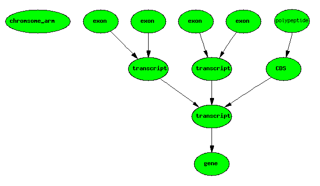
Other cases of trans-splicing may involve spatially distributed primary transcripts.
Feature Graph Transformations
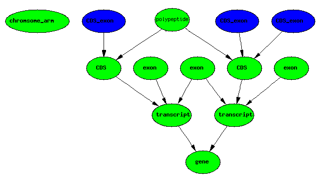
CDS boundaries + exons IMPLIES CDS exons
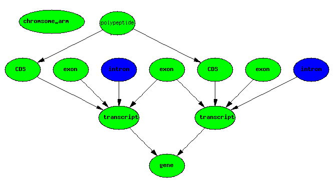
exons IMPLIES introns
Representing Graphs in a Relational Database
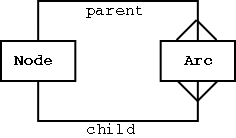
A graph can be defined as a collection of Edges (arcs) and Vertices (nodes).
Two table structure required for representing graphs
Representing Ontology Graphs in Chado
cvterms (controlled vocabulary terms) connected by cvrelationships
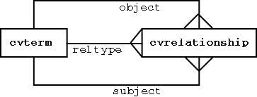
The relationship type is a controlled term in itself. Each cvrelationship can be thought of as a SUBJECT PREDICATE OBJECT statement (eg “GPCR is-a transmembrane_receptor).
The structure above is exactly the same as the RDF datamodel - many modern ontology languages (eg DAML, OWL) are layered on top of RDF, so the above structure ensures we will be able to represent all the most advanced ontological concepts.
Representing Feature Graphs in Chado
features are the nodes - feature_relationships are the arcs

Note: the different classes of features could be modeled relationally; the principle is to keep the stable stuff modeled relationally, and the fluid/extensible stuff modeled in an ontology that sits in a generic database structure.
Features are typed

Querying Graphs
Most implementations of SQL are non-recursive.
Problem: find all genes; find all genes (generic) find all noncoding genes find all protein coding genes find all tRNA genes find all snRNA genes find all snoRNA genes …etc eek!
Solution: pre-compute
transitive closure
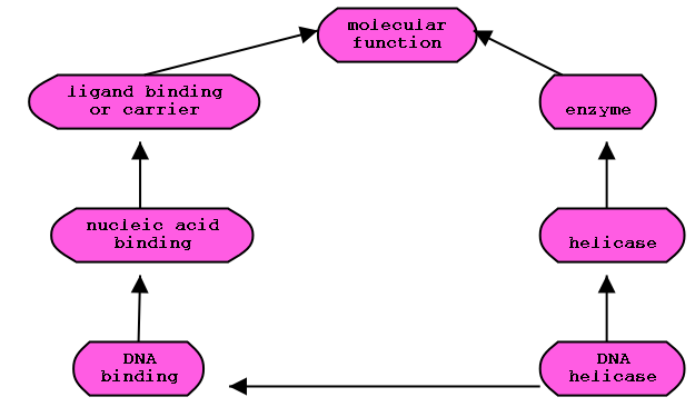
GO Ontology subgraph
Transitive closure of graph:
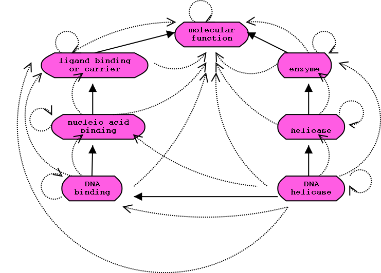
Solid lines represent the actual relationships. The collection of dotted
lines is the closure of the relationships.
forall x      ALWAYS TRUE:     x R* x

x R y             IMPLIES:     x R* y

x R y,  y R* z    IMPLIES:     x R* z
Using views to simplify queries
The following view uses the cvpath table, which includes the closure of the is_a relationship.
 CREATE VIEW fgene AS
   SELECT
     feature.*
   FROM
     feature INNER JOIN cvpath ON (feature.ftype_id = cvpath.subjterm_id)
     INNER JOIN cvterm ON (cvpath.objterm_id = cvterm.cvterm_id)
   WHERE cvterm.termname = 'gene';
At Flybase we will mostly be using chado in data-mining mode - i.e. we will be querying, not updating. This means we can materialize views for speed.
Extensible Attributes
The chado relational model defines a fixed set of attributes for a feature:
| Field | Required | Description |
|---|---|---|
| dbxref_id | no | namespaced identifier (foreign key) |
| name | no | A not-guaranteed-unique identifier that is useful to a human |
| uniquename | yes | name or identifier that is unique in the database |
| residues | no | DNA, RNA or protein sequence |
| md5checksum | no | signature of sequence |
| seqlen | no | length of sequence (may be present even if residues is absent) |
| type_id | yes | <a href=”http://sequenceontology.org” class=”external text” |
| rel=”nofollow”>Sequence Ontology</a> feature type (foreign key) |
What happens if we want to include other attributes specific to certain projects, or specific to certain feature types? We can use an extensible feature property paradigm:
We can attach any properties we like to feature:

Localising Features in Sequence Coordinates
All sequence localisations are with respect to another feature.
A feature can have multiple locations - however, “split” locations are not used (for an example of a split location, look at how Genbank represents a transcript).
Any feature can have 0 to many locations:

Each location is relative to another feature (the srcfeature)
The featureloc table includes the following attributes:
- fmin - 5’ boundary of features
- fmax - 3’ boundary of features
- strand: the direction of the feature, relative to srcfeature
locations have directional semantics (like mathematical vectors). this is different from the min/max semantics used by e.g. Bioperl, genbank
Interbase Coordinates
Chado uses interbase coordinates.
Interbase counts spaces, not bases. It is a 0-based coordinate system; counting starts at zero. This coordinate system is appealing for a variety of mathematical reasons. Standard (eg genbank, blast) coordinate systems do not allow for a natural representation of zero-length features. An example of a zero-length feature is a cleavage site that is between, but does not include, 2 amino acids. Using interbase coordinates the total number of base pairs in a feature is calculated by subtracting the starting coordinate from the ending coordinate, without the need for an off-by-1 addition required by other coordinate systems. (In general, much mathematical utility is enabled by the number zero.)
Interbase coordinates (top) and base-oriented (below)
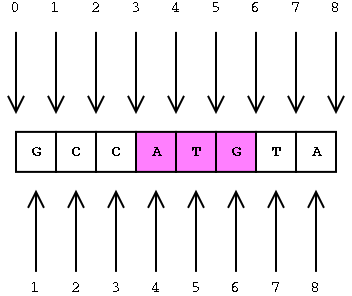
The position of the ATG in interbase is [3, 6] (between the 3rd and
6th gaps)
The position of the ATG in base coordinates is [4, 6] (between 4th and
6th bases inclusive)
Note the different arithmetic for calculating length in these two systems.
Unlike mathematical vectors, we must also explicitly store the directionality (strand). Even though this is surplus to requirements most of the time, it is required for zero-length features, and for circular chromosomes.
Basic example - with locations
Central dogma - with exons and CDSs localised
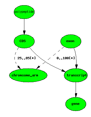
Using the principle of minimal storage (do not store anything that does
not increase the information content of the database - i.e. nothing
redundant), we store only exon and CDS boundary localisations. In the
Berkeley Drosophila Genome Project (BDGP) data
warehouse instantiation of Chado, we may choose to store locations for
all features where known - this can vastly simplify some queries, but
care must be taken to make sure we don’t end up with inconsistent data.
For the most part, infering the boundaries of composite features requires fairly simple graph transformations, although care must be taken for the genes that break central dogma rules.
Locations can be nested
A repeat localised to a contig, itself on a chromosome arm
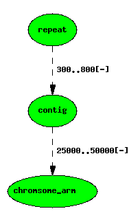
featurelocs are represented by dashed lines.
Note that the position of the repeat on the chromosome arm is implicit, and can be calculated with a simple graph transform, but following the principle of minimal storage, we do not store this in the management database.
If we wish to store the redundant position in a for-querying copy of the db, chado allows us this option - we can have as many locations as we like for a feature. We use an extra attribute called locgroup to distinguish locations. locgroup=0 is conventionally used for the non-redundant location.
The repeat feature now has two locations
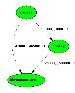
If you look at the underlying data, you will see that the featureloc
that locates the repeat on the arm has a locgroup values of 1.
Computational analysis: Predictions
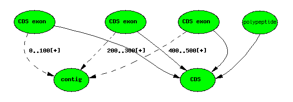
All predictions are handled analagously to standard central dogma cases. Compute results have scores, and are attached to tuples in the analysis table - this is what distinguishes them from “annotations”.
Genscan predicts CDSs and CDS exons (not genes in the Sequence Ontology sense). A typical Genscan prediction may look like this:
Genscan 3-exon ‘gene’ prediction
Computational analysis: Similarity results
Pairwise similarities (e.g. BLAST) and multiple alignments (e.g. CLUSTAL) are represented differently.
Pairwise alignments produce HSPs. HSPs are scored features with two locations - one on the query, one on the subject.
Blast hit with 3 HSPs

Each HSP has two featurelocs. featureloc has an attribute rank to
order the locations; by convention 0 is the query rank and 1 is the
subject rank.
Computational analysis: Multiple alignments
These are treated analagously to pairwise alignments - just add more locations.
Variation features
Variation features (e.g. SNPs, insertions, deletions) are treated in a similar fashion to pairwise alignments.
Bioperl and chado mapping
There are important differences between the Bioperl and chado models.
Bioperl allows a feature to have multiple non-contiguous locations. Even though the chado schema allows multiple locations, attaching multiple non-contiguous locations is a violation of the chado semantics. To cope with this, we create extra features for the sublocations. For instance, for a transcript, we would create an exon for each of the sublocations.
If you parse a genbank file including variations (e.g. SNPs) into Bioperl objects, you will get a feature with two properties of type “allele”. This can be represented using chado; however, the chado semantics state that these variations should be represented using multiple locations.
Acknowledgements
Schema design
- Dave Emmert
- Colin Wiel
- Stan Letovsky
- ShengQuiang Shu
- Pinglei Zhou
- Suzanna Lewis
Chado beta testers and other feedback
- Mark Yandell
- Aubrey de Grey
About this Page
- This page is a Wikified version of a presentation by Chris Mungall.