GMOD
JBrowse2 Tutorial PAG 2024
This tutorial will be/was presented at the Plant and Animal Genomes conference on January 14, 2024. After the tutorial is over, a public Ubuntu AMI that was used for the tutorial will be available for anyone who would like to work through the tutorial afterwards.
Contents
- 1 Running an instance of the tutorial AMI
- 2 Prerequisites (already installed)
- 3 Initializing JBrowse
- 4 Adding a reference sequence
- 5 Adding a gene track from tabix-indexed GFF
- 6 Adding text search indexes
- 7 Adding a gene track from a JBrowse (NCList) track
- 8 Adding BAM/CRAM data
- 9 Adding variant data from a tabix-indexed VCF
- 10 Adding quantitative data from a BigWig
- 11 Adding a track with multiple BigWigs
- 12 Working with metadata and facets
- 13 Synteny
- 14 Using the Structural Variant Inspector
- 15 Using JEXL to modify the display
- 16 Using the admin-server
Running an instance of the tutorial AMI
To run this tutorial on your own Amazon EC2 instance, use ami-0982eea63d790bad6 in the us-east-1 region.
There are several things to know about this instance:
- It is Ubuntu 22.04 LTS with the login user account ubuntu
- As long as you don’t plan on running things like minimap2 (which you don’t need for the tutorial), you can run this instance as a t2.micro and probably even as a t2.nano instance
- In your security groups, open up ports for ssh (22) and http (80), and if you want to use the jbrowse admin server, open port 9090.
- To make life easier on you, you can add an entry in your client machine’s /etc/hosts file for the IP address of the EC2 machine that resolves for tutorialpag31.jbrowse.org. If you don’t do this, you’ll have to use the IP address of your EC2 machine in the URLs in this tutorial instead of “tutorialpag31.jbrowse.org”.
- The easiest way to do the tutorial is with the ubuntu user, and your instance of JBrowse would then be at http://tutorialpag31.jbrowse.org/~ubuntu
Prerequisites (already installed)
- NodeJS
Installed using the instructions on Nodejs.org:
 Don't do:
 $ curl -fsSL https://deb.nodesource.com/setup_18.x | sudo -E bash - &&sudo apt-get install -y nodejs
- A web server (Apache2 in this instance, but any will do). I enabled the “userdir” mod so we could all use the same machine for the tutorial:
 Don't do:
 $ sudo a2enmod userdir
 $ sudo service apache2 start
Things done just for this tutorial
- A script to create several users with
public_htmldirectories - Already installed the
JBrowse command line interface (CLI) via the
directions (i.e.,
sudo npm install -g @jbrowse/cli) - Installed bgzip, tabix, samtools and minimap2 via apt:
sudo apt-get install samtools tabix minimap2. - Created a bgzipped and samtools faidx’ed FASTAs file for C. elegans and C. brenneri.
- Created a “Genes only” C. elegans GFF file
(
gzip -dc c_elegans.PRJNA13758.WS286.annotations.gff3.gz | grep "\tWormBase\t" > c_elegans.genes.gff3) - Created a bash script that will do all of the commands in this tutorial “all at once”.
Initializing JBrowse
First, use ssh or putty to connect to the instance we have set up for this tutorial, tutorialpag31.jbrowse.org. Do this with the user name and password you got from one of us (we have 50 users configured–hopefully that will be enough!):
ssh username@tutorialpag31.jbrowse.org
and supply the password. When you log in, you’ll be in your user’s home directory, where there is nothing but a public_html directory. We’ll use the JBrowse CLI to initialize a new JBrowse instance:
 jbrowse create public_html --force
 cd public_html
Note that the “–force” is necessary here because the public_html
directory isn’t empty and the create script doesn’t want to accidentally
delete any existing files. We’re safe though. Now change to that
directory, cd public_html and do a file list to make sure it looks
right:

This is all of the software required to run JBrowse, plus soft links to files we are going to use in the tutorial. If we now navigate to the tutorial machine’s website with the username on the slip provided at the beginning, you should see a page indicating that JBrowse was installed but not configured: http://tutorialpag31.jbrowse.org/~userXX. (Of course, substitute in your username in the URL)

To make sure it really works, we can click on the Volvox (not really Volvox) data set.
Adding a reference sequence
The first thing we need to do is add a reference sequence. There is a samtools/faidx indexed fasta file already in your public_html directory. To create this indexed reference sequence, the fasta was downloaded from the WormBase ftp site, and after uncompressing it, it was bgzipped and then indexed with SAMTools:
 Don't do:
 bgzip c_elegans.PRJNA13758.WS286.genomic.fa
 samtools faidx c_elegans.PRJNA13758.WS286.genomic.fa.gz
To tell JBrowse about the new assembly, we can use the jbrowse CLI:
 jbrowse add-assembly data/c_elegans.PRJNA13758.WS286.genomic.fa.gz \
         --displayName "C. elegans N2" \
         --name c_elegans_PRJNA13758 \
         --type bgzipFasta \
         --load inPlace \
         --refNameAliases data/ce_aliases.txt
The command will probably generate some warnings about the locations of
the files, but the apache server is configured to use them where they
are (i.e., FollowSymLinks was added to the configuration).
In this command, --displayName is what will appear in the user
interface, --name is what will be used in future configuration options
to refer to this assembly, --type refers to how the fasta file was
indexed, and --load inPlace tells the CLI to leave the files where
they are (other options include “copy”, “symlink” and “move”). The
--refNameAliases option gives options for how chromosomes are named;
that will be covered in more detail below. Note that we don’t specify
the location of the .fai and .gzi files in this command; the CLI will
assume the names from the name of the compressed fasta file (it is
possible to specify them on the command line too if they aren’t
“guessable”). Copy this command and run it in the public_html directory.
After doing that, go to the web browser and if you aren’t on the splash
screen, select “Return to splash screen” from the file menu, and start a
new session and then launch a LinearGenomeView. You should get a dialog
to open an assembly with “C. elegans N2” as the only option.

Go ahead and open chromosome I.
Adding a gene track from tabix-indexed GFF
GFF3 is a very common file format for defining genome features. The GFF3 file we’re using today is based on the on created by WormBase for every release. Here is a sample:
  I WormBase    gene    4116    10230   .   -   .   ID=Gene:WBGene00022277;Name=WBGene00022277;locus=homt-1;sequence_name=Y74C9A.3;biotype=protein_coding;so_term_name=protein_coding_gene;curie=WB:WBGene00022277;Alias=homt-1,Y74C9A.3
  I WormBase    mRNA    4116    10230   .   -   .   ID=Transcript:Y74C9A.3.1;Parent=Gene:WBGene00022277;Name=Y74C9A.3.1;wormpep=CE28146;locus=homt-1;uniprot_id=Q9N4D9
  I WormBase    three_prime_UTR 4116    4220    .   -   .   Parent=Transcript:Y74C9A.3.1
  I WormBase    CDS 4221    4358    .   -   0   ID=CDS:Y74C9A.3;Parent=Transcript:Y74C9A.3.1;Name=Y74C9A.3;prediction_status=Confirmed;wormpep=CE28146;protein_id=CCD68263.1;locus=homt-1;uniprot_id=Q9N4D9
  I WormBase    intron  4359    5194    .   -   .   Parent=Transcript:Y74C9A.3.1;Note=Confirmed_EST yk1692c07.3 %3B Confirmed_EST OSTR037H1_1 %3B Confirmed_EST elegans_PE_SS_GG2157%7Cc1_g1_i1 %3B Confirmed_EST elegans_PE_SS_GG2157%7Cc1_g1_i1 %3B Confirmed_EST adult_Nanopore_Roach_35350 %3B Confirmed_EST adult_Nanopore_Roach_35350 %3B Confirmed_EST adult_Nanopore_Roach_35350 %3B Confirmed_EST adult_Nanopore_Roach_35350 %3B
  I WormBase    CDS 5195    5296    .   -   0   ID=CDS:Y74C9A.3;Parent=Transcript:Y74C9A.3.1;Name=Y74C9A.3;prediction_status=Confirmed;wormpep=CE28146;protein_id=CCD68263.1;locus=homt-1;uniprot_id=Q9N4D9
One of the easiest ways to use GFF3 with JBrowse is to use a tabix indexed bgzipped file. Generally, before creating the tabix index, GFF3 files have to be sorted first by the reference sequence (ie, the chromosome name, in column 1) and then by the starting coordinate (colunn 4). Here is a magic incantation for doing that on the Linux command line (sort and then pipe the result to bgzip):
 Don't do:
 sort -t"`printf '\t'`" -k1,1 -k4,4n c_elegans.genes.gff3 |bgzip > c_elegans.genes.sorted.gff3.gz
Note that this command, while it will work, is perhaps a little over simplistic. See the JBrowse website for a little more information on preparring GFF3 files.
Then tabix index it:
 Don't do:
 tabix c_elegans.genes.sorted.gff3.gz
To save time, we placed both the bgzipped GFF and tabix index files in your public_html directory as well. To use the CLI to add a GFF track, do this:
 jbrowse add-track data/c_elegans.genes.sorted.gff3.gz \
         --name Genes \
         --description "Curated genes from WormBase" \
         --load inPlace \
         --config '{ "metadata": { "source":"GFF3 created by Scott Cain, from WormBase annotation file at https://downloads.wormbase.org/releases/WS286/species/c_elegans/PRJNA13758/c_elegans.PRJNA13758.WS286.annotations.gff3.gz" } }'
Where the options are the same as before, with the --description
option to provide information about what the track is. Additionally, we
added a metadata block with the --config option, which allows us to
add any json formatted section to the resulting track configuration.
Reload the page in the web browser and open the track selector if it
isn’t already open, and select the “Genes” track. Note that when you
hover your mouse over the Genes track checkbox, the description appears
in a tooltip.
Adding text search indexes
The jbrowse CLI provides tools to create text indexes of many of the
data sources we used, like tabix indexed files. Note that it does not
index JBrowse 1 (NClist) data;
that is somewhat more complicated and out of scope for this tutorial. We
can create a searchable index for the Genes track we created. To do
that, on the command line in the public_html directory, run the command
jbrowse text-index --attributes=Name,ID,locus --tracks c_elegans.genes.sorted.gff3
The default value for the attributes flag are “Name,ID” so it will index the GFF attributes that have those tags. For this command, we add the “locus” attribute, because WormBase puts the “human readable” name in that attribute.
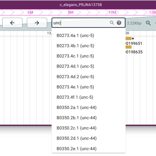
After this command completes, we can reload our browser window and type something in the search box (ie, the text field where the location is typically displayed). Try your favorite worm gene (worm genes are usually three characters plus a hyphen plus a number). Try “unc” if nothing else comes to mind.
Adding a gene track from a JBrowse (NCList) track
Another sort of data that can be used with JBrowse 2 is data that is
currently being used with JBrowse 1. The most common way GFF data is
used with JBrowse 1 is via processing with the flatfile_to_json.pl
script that generates a set of data files that are collectively referred
to as NCList (Nested Containment List). At WormBase there is a JBrowse 1
instance with many such tracks. We’ll use one of those as an example
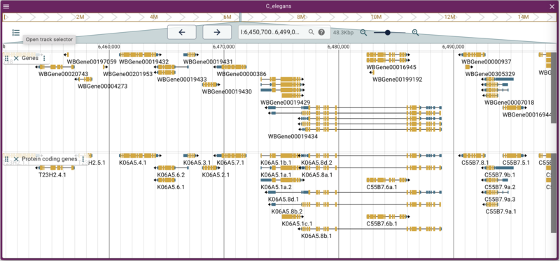
here to load a track that has just protein coding genes:
 jbrowse add-track https://s3.amazonaws.com/agrjbrowse/MOD-jbrowses/WormBase/WS286/c_elegans_PRJNA13758/tracks/Curated%20Genes%20\(protein%20coding\)/{refseq}/trackData.jsonz \
   --name "Protein coding genes" \
   --description "Only protein coding genes from WormBase" \
   --config '{ "metadata": { "source":"Directly from WormBases JBrowse 1 instance at https://wormbase.org/tools/genome/jbrowse" } }'
Note that the –load option isn’t required for URLs.
Side note: finding JBrowse 1 data
While JBrowse 1 instances are plentiful, there are a few tricks for finding those data. First, in JBrowse 1, you can always open the “Edit config” for a track to get the details of where the data are coming from (look for the urlTemplate entry).
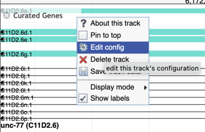
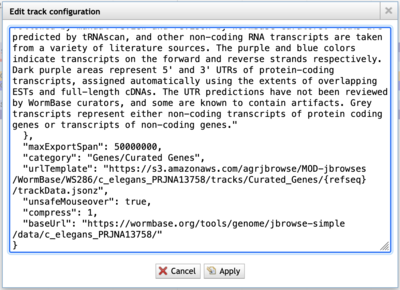
If the urlTemplate entry is a relative URL, you’ll have to combine that with the base URL to get an absolute URL to use with JBrowse 2. Additionally, if the admin of the JBrowse 1 instance that you’re getting data from doesn’t have CORS (Cross-Origin Resource Sharing) turned on, the data will fail to load in JBrowse 2. Frequently, a polite request will get CORS turned on.
Also, this is one difference between the web and desktop versions of JBrowse 2, since there is no such CORS limitation on the desktop version. That is, if you can figure out the URL of the data, you can use it in the desktop version no matter what.
Adding BAM/CRAM data
The C. elegans Natural Diversity Resource (http://elegansvariation.org/) creates read and variant data for many strains of C. elegans and makes them available to the research community. An example of the read data they provide is this BAM file for the CB4854 strain. To load a BAM file, we simply provide a URL for the file and give the track a name:
 jbrowse add-track https://s3.amazonaws.com/agrjbrowse/MOD-jbrowses/WormBase/static_tracks/modencode-bucket/test/CeNDR/CB4854.bam \
       --name "CeNDR BAM" \
       --config '{ "metadata": { "source":"Used by permission from http://elegansvariation.org/" } }'
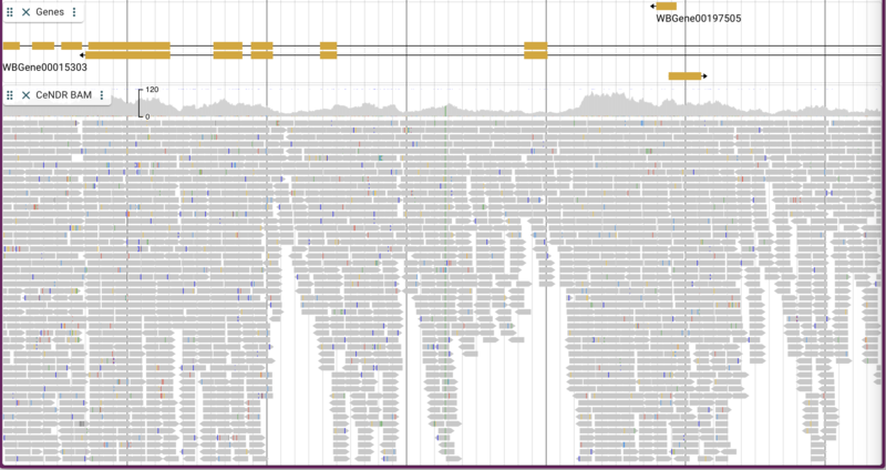
By default, both the coverage plot and individual alignments are shown with mismatches highlighted and “going up” to the coverage plot.
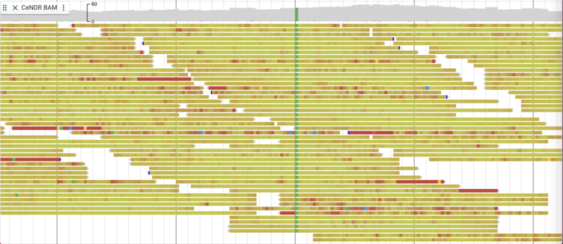
There are a few nice things to point out about the way alignment data are presented. You have the option of turning on and off both the individual alignment sections and the coverage sections as well as changing many attributes relating to the overall display. To make changes in the display, click on three vertical dots in the track label to get a drop down menu with many options. For example, you can change the coloring of the glyphs according to a variety of parameters. Below is is an example with the “per base quality” coloring turned on:
Adding variant data from a tabix-indexed VCF
Variant data from VCF files can be added in much the same way the tabix
index GFF and BAM files are added. Typically, the VCF files need to be
sorted, bgzipped and tabix indexed in pretty much the same way as GFF
(the Linux sort command is slightly different but that’s it), but in
this case, there is an already indexed file for wild variants of C.
elegans sitting in a Google API share (which already has CORS enabled).
These data a provided by the C. elegans Natural Diversity Resource
(http://elegansvariation.org/) as well. Adding it is
very simple, just supplying the URL of the file and a name for the
track:
 jbrowse add-track https://storage.googleapis.com/elegansvariation.org/releases/current/WI.current.soft-filtered.vcf.gz \
         --name Variants \
         --config '{ "metadata": { "source":"Used by permission from http://elegansvariation.org/" } }'
The result up to this point looks something like this:

Adding quantitative data from a BigWig
Adding other types of binary data files like BigWig and BigBed are also straight forward. Again, there is a set of BigWig files for C. elegans that are served from the Broad Institute that uses conservation data across several species to predict what reading frame is being used in an exon. Using the link for the frame one prediction, we can write a command that is again very similar to the previous commands:
 jbrowse add-track https://data.broadinstitute.org/compbio1/PhyloCSFtracks/ce11/latest/PhyloCSF+1.bw \
   --name "Frame 1 usage" \
   --config '{ "metadata": { "source":"Publicly available data from the Broad Institute: https://data.broadinstitute.org/compbio1/PhyloCSFtracks/trackHub/mm39/PhyloCSF_raw.html" } }'

The need for alias files
This example is slightly different, though it doesn’t look like it here. The problem is one of the plagues of bioinformatics: how people name things. At WormBase, chromosomes are named with Roman numerals: I, II, III, etc, but at UCSC, they are named with a “chr” prefix: chrI, chrII, chrIII, etc. This presents somewhat of a problem for genome browsers, since the “name” of the location (like “I:12345..44345”) is pretty fundamental to how they work. In the case of this data from the Broad (and for that matter, any data we might want to get from UCSC), they use the “chr” prefix. Fortunately, JBrowse has a way to deal with that, which is providing a file that has aliases. An alias file like the one we specified when we added the C. elegans reference sequence set is just a comma delimited text file with the “canonical” names of the reference sequences with “alternate” names in subsequent columns, like this:
I   chrI    ChrI
II  chrII   ChrII
III chrIII  ChrIII
IV  chrIV   ChrIV
V   chrV    ChrV
X   chrX    ChrX
MT  chrM    M   ChrM
Of course, “chr” isn’t the same as “Chr” either. When we added the
reference sequence, I knew this was going to be an issue, so we added
--refNameAliases data/ce_aliases.txt to the command.
Adding a track with multiple BigWigs
The JBrowse command line interface makes adding many track types very
easy, but also allows us to do more complicated things if we know what
we’re doing. Adding a track with multiple BigWigs is one such example.
Up to now, we been using the add-track option, but there is also a
add-track-json option that will add “naked” json to our configuration.
An example of what the json configuration for a multiple BigWig track looks like this:
    {
      "type": "MultiQuantitativeTrack",
      "trackId": "multiwiggle_phylo",
      "name": "Forward PhyloCSF",
      "assemblyNames": [
        "c_elegans_PRJNA13758"
      ],
      "adapter": {
        "type": "MultiWiggleAdapter",
        "bigWigs": [
          "https://data.broadinstitute.org/compbio1/PhyloCSFtracks/ce11/latest/PhyloCSF+1.bw",
          "https://data.broadinstitute.org/compbio1/PhyloCSFtracks/ce11/latest/PhyloCSF+2.bw",
          "https://data.broadinstitute.org/compbio1/PhyloCSFtracks/ce11/latest/PhyloCSF+3.bw"
        ]
      },
      "metadata": {
        "source" : "Publicly available data from the Broad Institute: https://data.broadinstitute.org/compbio1/PhyloCSFtracks/trackHub/mm39/PhyloCSF_raw.html"
      },
      "displays": [
        {
          "type": "MultiLinearWiggleDisplay",
          "displayId": "multiwiggle_phylo-MultiLinearWiggleDisplay"
        }
      ]
    }
which I created in the JBrowse desktop application and then just copied and pasted the resulting config here. To use this with the JBrowse CLI, we just need to make it “command line friendly” (ie, put it all on one line and put it in single quotes):
jbrowse add-track-json '{"type":"MultiQuantitativeTrack","trackId":"multiwiggle_phylo","name":"Forward PhyloCSF","assemblyNames":["c_elegans_PRJNA13758"],"adapter":{"type":"MultiWiggleAdapter","bigWigs":["https://data.broadinstitute.org/compbio1/PhyloCSFtracks/ce11/latest/PhyloCSF+1.bw","https://data.broadinstitute.org/compbio1/PhyloCSFtracks/ce11/latest/PhyloCSF+2.bw","https://data.broadinstitute.org/compbio1/PhyloCSFtracks/ce11/latest/PhyloCSF+3.bw"]},"metadata":{"source":"Publicly available data from the Broad Institute: https://data.broadinstitute.org/compbio1/PhyloCSFtracks/trackHub/mm39/PhyloCSF_raw.html"},"displays":[{"type":"MultiLinearWiggleDisplay","displayId":"multiwiggle_phylo-MultiLinearWiggleDisplay"}]}'
Yes, that is a ridiculously long command. The result with all three bigwigs in one track looks like this:

Note that I use this method of creating tracks pretty frequently: I figure out what I want it to look like in the JBrowse desktop application and then when it’s ready, I copy and paste the track config into my website config.
Working with metadata and facets
All of the tracks we’ve added up to this point have included a “metadata” section. JBrowse provides a faceted browser that allows users to filter tracks by the metadata that you provide. To find the faceted browser, click the “hamburger menu” next to the “filter tracks” field at the top of the “Available tracks” panel:
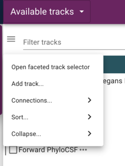
In the resulting dialog, the facets that are provided in the configuration are selectable (with multiple selections available with shift-click) to limit tracks shown. Of course, since we don’t have that many tracks, this is a limited example, but when there are dozens or hundreds of tracks, this provides a way to help users find the data they want.

Synteny
To compare two genomes, first we need a second genome. Fortunately, WormBase.org provides several assemblies for species related to C. elegans. For this tutorial, we’ll use C. briggsae. As before, we create a new assembly in JBrowse with the indexed fasta files provided on the tutorial machine:
jbrowse add-assembly data/c_briggsae.PRJNA10731.WS287.genomic.fa.gz \
        --displayName "C. briggsae" \
        --name c_briggsae_PRJNA10731 \
        --type bgzipFasta \
        --load inPlace
Next we need some analysis result that compares the two genomes. The
tool minimap2 is a fairly lightweight application that will do a fast
comparison and generate a PAF file (other formats that JBrowse supports
include anchors files from MScanX, out files from MashMap, and delta
files from Mummer). I ran this command ahead of time and put the result
in the public_html directory:
 Don't do:
 minimap2 -c data/c_elegans.PRJNA13758.WS286.genomic.fa.gz data/c_briggsae.PRJNA10731.WS287.genomic.fa.gz > c_elegans.c_briggsae.paf
Note the use of the -c flag: that adds CIGAR information to each of the match lines, which JBrowse will use to improve the display with insertion and deletion data. Once we have the paf file, we can create a tabix index and add it to JBrowse.
Tabix indexing of PAF file
The original design of JBrowse synteny tracks required that an entire
comparative genome result be loaded. Since those can be quite large, we
developed a method of compressing and indexing PAF files that is similar
to what you might have with GFF or VCF indexed files that we are giving
the file extension .pif. Using indexed PAF files can significantly
reduce the load time for pages by an order of magnitude or more, though
since these genomes are fairly small the difference in load times would
also be small. To create this indexed PAF file, use the make-pif
option of the jbrowse cli:
jbrowse make-pif data/c_elegans.c_briggsae.paf
which will create two files: c_elegans.c_briggsae.pif.gz (the
block-compressed PAF file) and c_elegans.c_briggsae.pif.gz.tbi (the
index file). We can now use this indexed file to create a synteny track
with the jbrowse cli like this:
 jbrowse add-track c_elegans.c_briggsae.pif.gz \
     --assemblyNames c_briggsae_PRJNA10731,c_elegans_PRJNA13758 \
     --description "A minimap2 comparison of C. elegans and C. briggsae" \
     --load inPlace \
     --name "C. elegans/C. briggsae Synteny" \
     --config '{ "metadata": { "source":"Comparative analysis using this command: minimap2 -c data/c_elegans.PRJNA13758.WS286.genomic.fa.gz data/c_briggsae.PRJNA10731.WS287.genomic.fa.gz > c_elegans.c_briggsae.paf" } }'
A new flag for this command is --assemblyNames; in previous commands
adding a track, the assembly that was being used was inferred to be the
default (and only up to that point) assembly. Now that we are comparing
two assemblies, we have to be explicit about what assemblies we are
comparing. Also, one thing that has tripped me up a few times is that
the order of the assemblies in this command matter, and is the opposite
of the order that they occur in the minimap2 command. If you try to do
something like this and don’t get an error in JBrowse but also get an
empty track, try the command again, switching the order of the
assemblies in the --assemblyNames flag.
Adding a gene track for C. briggsae
To make the synteny display a little more informative, we’ll also add a gene track for the C. briggsae assembly (so we can see what’s being compared):
 jbrowse add-track https://s3.amazonaws.com/agrjbrowse/MOD-jbrowses/WormBase/WS287/c_briggsae_PRJNA10731/tracks/Curated_Genes/{refseq}/trackData.jsonz \
     --assemblyNames c_briggsae_PRJNA10731 \
     --name "C. briggsae Genes" \
     --trackId c_briggsae_genes \
     --config '{ "metadata": { "source":"Curated genes track directly from the WormBase JBrowse 1 instance." } }'
Opening a synteny display
When we reload JBrowse, we’ll now have a track called “C. elegans/C. briggsae Synteny” and when we turn that on, we’ll see regions in the C. elegans genome that have synteny to the C. briggsae genome. If we right click on one of those regions and select the option from the popup menu, it will open a new synteny display. After opening the gene tracks for each assembly, it will look something like this:
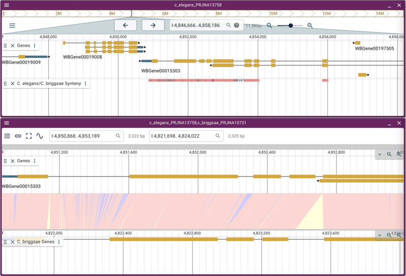
Note that the pink/salmon colored synteny regions in the linear genome view’s synteny track indicate that the matching region is in the same orientation whereas a purplish-blue region indicates match regions that are in opposite orientations.
Using dotplot and synteny views
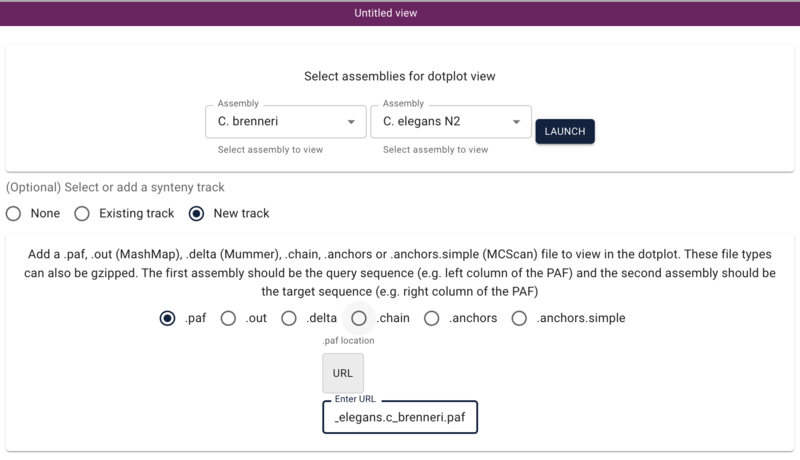
Another way we can visualize comparative data is via a dotplot. If we return to the JBrowse splash screen (via the File menu) and select “Start a new [empty] session” we get the “Select a view to launch” menu with LinearGenomeView as the default. Selecting instead DotplotView, we get a dialog that offers to start a new dotplot. Select C. elegans in the first drop down and then C. briggsae in the second (again, order matters) and click the “Existing track” radio button if it’s not already selected. If “Existing” wasn’t already selected, the dialog will change to show a drop down menu with only one entry for our newly created synteny track (otherwise it should already be there). Click “Launch.”
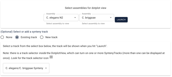
That will create this moderately messy dotplot (at least we can see there are regions in corresponding chromosomes that have synteny!):
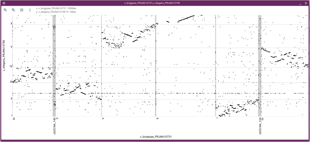
We can either zoom in or open a synteny view by using the mouse to select a rectangular region in the dot plot. Selecting a region of fairly long synteny in C. elegans chromosome II and going to the synteny view gives us something like this:
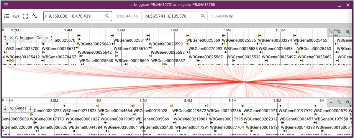
Note that when we have crossing synteny blocks, we can horizontally flip one of the tracks (so it’s decreasing coordinates from left to right rather that the default increasing left to right) by accessing the menu in the up left corner of the frame.
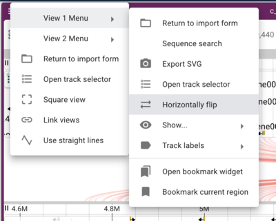
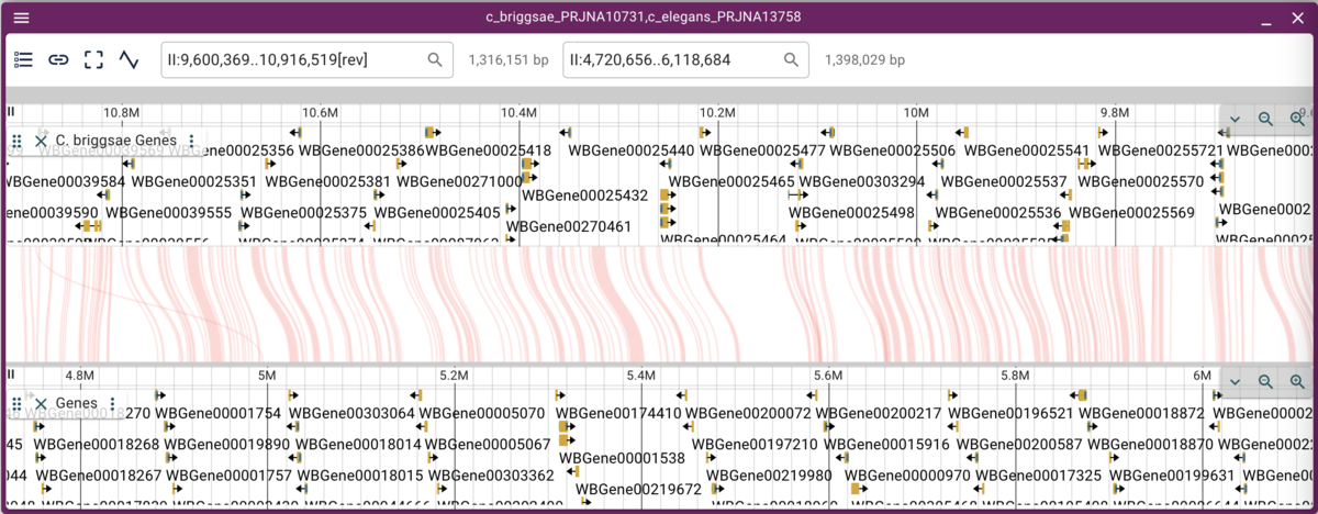
Now we can more easily zoom into regions we might be interested in.
Using the Structural Variant Inspector
JBrowse’s SV Inspector takes a set of structural variant predictions from BAM files with either long or short reads, with support for Manta, Delly, Lumpy (short reads); and pbsv, Sniffles (long reads). The resulting prediction file can be loaded via the “New session” dialog and selecting SVInspectorView from the menu.
In the resulting dialog, we can use a Manta-generated set of SV predictions comparing a C. elegans strain (VC109) to the N2 workhorse strain. This experiment was performed by Maroilley et al with short reads. To start, we can use this url for the Manta VCF file:
https://s3.amazonaws.com/agrjbrowse/MOD-jbrowses/WormBase/static_tracks/modencode-bucket/test/maroilley/candidateSV.vcf.gz
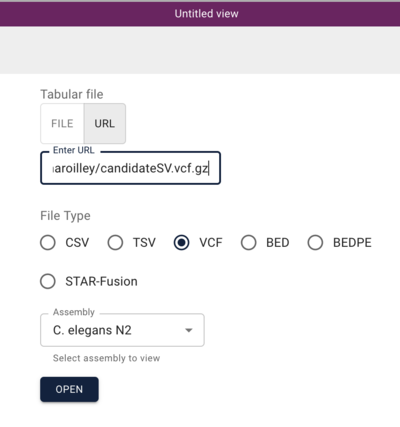
And when we click “Open”, we get a view that has a spreadsheet of the predictions and a circular genome view with arcs drawn for the predicted variants.
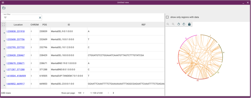
To make full use of this view, though, we need two tracks: one for the source BAM file and one for the predictions VCF. To get them, run these load-track commands:
 jbrowse add-track https://s3.amazonaws.com/agrjbrowse/MOD-jbrowses/WormBase/static_tracks/modencode-bucket/test/maroilley/candidateSV.vcf.gz \
       --name "Structural Variant Candidates VCF" \
       --assemblyNames c_elegans_PRJNA13758 \
       --category "Structural Variants"


 jbrowse add-track https://s3.amazonaws.com/agrjbrowse/MOD-jbrowses/WormBase/static_tracks/modencode-bucket/test/maroilley/VC109_Het_trim_bwaMEM_sort.bam \
       --name "VC109 BAM" \
       --assemblyNames c_elegans_PRJNA13758 \
       --category "Structural Variants"
Note that these load commands have a option we haven’t seen yet:
--category, which will put the newly created tracks in a separate
section in the track list to make them easier to find. Also note that we
have to provide the name of the assembly that these files use as a
reference, since we have two now. After running these commands, reload
the JBrowse page to make sure the new configuration is available.
Now we’d like to find a set of regions to inspect. We can click on any of the arcs to get a set, but lets pick one region so we’re all looking at the same thing. The authors mention a rearrangement in the unc-36 gene, and we can filter the locations by region. To do that, click on hover dropdown triangle in the Location column header (that is, put your mouse over the Location header to get the triange to appear, then click on it) to get a menu, and select the “Create filter” option. Then paste in this location (the coordinates of the unc-36 gene to find overlapping predictions):
III:8,193,845..8,201,219
Which will give us just two rows. To select one of them (since they overlap in the circular view), we can highlight one row in the spreadsheet view and then that will be other only arc in the circular view. Finally, clicking on that arc gives us two stacked linear genome views of the two regions with the predicted rearrangement:

Now we can click on the open track selector buttons for each of the linear genome views, and open the BAM and VCF tracks for each, resulting in a view like this:
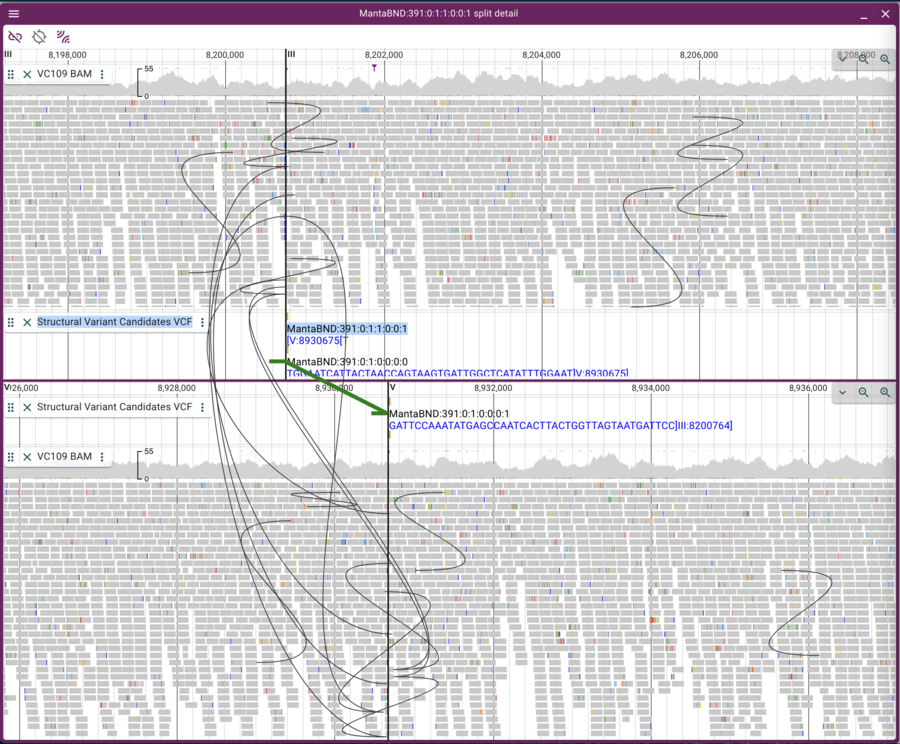
This view is a little messy because there are lots of curves showing pairs of reads that aren’t where we “expect” them to be. We can limit the view to only inter-chromosomal read pairs by clicking on the “two arc sets” button in the upper left of the frame.
Using JEXL to modify the display
JBrowse 2 has several tools available for changing the way things look (adding plugins, modifying the config.json manually to change things like highlight colors, etc) but one easily accessible method is using JEXL (JavaScript EXpression Language). If we were using the JBrowse desktop application or the admin-server, we could make these changes directly on the tracks we are creating, but since we are using the JBrowse web application as a “normal” user, we can only make changes to a personal copies of tracks. The process though is fundamentally the same in all cases.
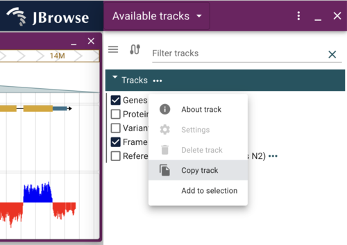
We will modify how the Genes track looks. To get started, we’ll make a copy of the track by clicking on the “…” after the name of the track in the track selector, and select “Copy track” from the drop down menu (again, with the desktop or admin-server, the “Settings” options wouldn’t be greyed out).
Dynamically changing the color
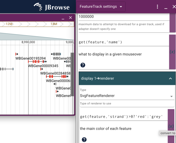
To start editing how our “local” copy of the Genes track looks, click the checkbox for our local track to turn it on and again click on it’s “…” and select “Settings”, which will open a new display where the track selector was. Scroll down until you see the “Display 1->renderer” section that starts with several color blocks, the first of which is my favorite color, goldenrod, which is the default primary color for discrete features like genes. To change that to some other color, we can do multiple things. First, we can just type the name of a different color. Pick one and see if it will work. We can also click on the color block to get a color picker to graphically pick any color we want. Note that any type we change the color, the change to the track happens instantaneously. Also note that if we change to a color that doesn’t exist (or do something else that doesn’t make “sense”), the color will change to black in the track.
To make a change that depends on the feature itself, we can use JEXL. To
start using JEXL for an display item, we first have to check the radio
button in the purply area to the right of the thing we want to change.
This text JBrowse that rather than interpreting what we write in the
text field as the name of a color (in this instance), we want it
interpreted as JEXL. In JBrowse, the JEXL commands typically start with
get(feature,'attribute) which allows us to get the value of anything
the JBrowse knows about a given feature. In this case, all of the gene
features have a “strand” attribute, and it is either 1 or -1. We can
write a statement at the uses the ternery operator (i.e., if the thing
before the ? is true, do the first thing, otherwise do the second thing)
that looks like this:
get(feature,'strand')>0?'red':'grey'
Enter that in the field where goldenrod used to be, and see the genes change to either red or grey depending on which strand they are on.
Dynamically changing the mouseover text
In the section just above where we change the colors in the “Display 1” section, we see an item that is already in JEXL:
get(feature,'name')
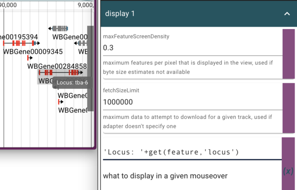
which is what gets displayed when you hover your mouse over a feature. In this case, the feature’s name is not terribly informative, so we’d like to change it. In addition to switching to using the feature’s “locus” attribute (which is where the human readable version of the gene’s name is), we’ll also add a text label to make it clear that’s where we got it. To do this, we can enter
'Locus: '+get(feature,'locus')
where the “name” JEXL was. This tells JBrowse to get the feature’s “locus” attribute and then prepend it with “Locus: “ in the tooltip.
Getting the config
One way I use for the settings editor for a copy of a track is to figure
out how the json for a particular change would look so that I can
incorporate it into tracks I’m writing “by hand” (that is, by editing
the config.json file by hand). To get the raw json for a track, you
can select the “About this track” from the “…” menu and then pressing
the “Copy config” button.

Pasting that into a text editor will give you the full track json:
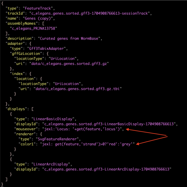
which shows how the changes we made in the user interface gets added to the site configuration.
Using the admin-server
 NOTE: This section will not be done in the live tutorial for a variety reasons, including
 that we don't have the ports open to run the admin server. This section is here to introduce
 the concept should you arrive at this page when not doing the tutorial.
We can also run the JBrowse admin-server, which looks just like JBrowse
proper, but has an extra admin menu. Important note: The admin
server is NOT meant to be left running; it is not particularly secure,
so if you leave it up, somebody might start messing with your site. To
start the admin server, we change to the directory where JBrowse will be
served from (public_html) and run the jbrowse command to start it:
jbrowse admin-server
When we execute that command, we get a message in the terminal that it started up and gives us some URLs to use to access the server. It will look something like this:

The part we need is the adminKey. In a browser window, enter a URL that looks like this: http://tutorialpag31.jbrowse.org:9090?adminKey=yourkey
Using the admin-server to add an assembly
The first thing we need to do is add a reference sequence. There is already one prepared and on the web server for C. elegans and it is at
 http://tutorialpag31.jbrowse.org/~ubuntu/data/c_elegans.PRJNA13758.WS286.genomic.fa.gz
 http://tutorialpag31.jbrowse.org/~ubuntu/data/c_elegans.PRJNA13758.WS286.genomic.fa.gz.fai
 http://tutorialpag31.jbrowse.org/~ubuntu/data/c_elegans.PRJNA13758.WS286.genomic.fa.gz.gzi
To add this as a reference sequence to JBrowse, click on the “Start a new session” and then on the resulting page, select “Open assembly manager” from the Admin menu. In the dialog that opens, click the “Add new assembly” button. Finally, in add assembly dialog, put something useful in the “Assembly Name” field and then select “BgzipFastaAdapter” from the “Type” menu. At that point, the dialog will change slightly to give you places to put in the above three URLs:
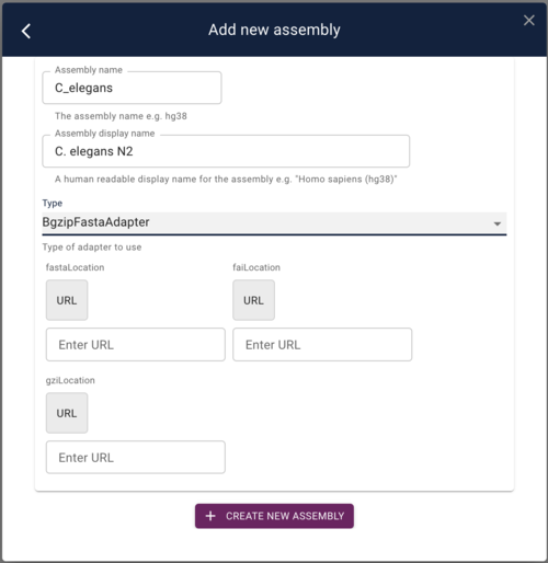
Copy and paste those URLs in to the appropriate fields and then click “Save new assembly.”
  Note: this is one place where the web version of JBrowse with the admin server is slightly
  different from the Desktop version: if we were using the desktop version, the above dialog
  would have also given the option for finding the files on a local hard drive rather than
  only allowing URLs.

  Another note: In order for the above URLs to work with a web instance of JBrowse that
  isn't on the "same" server (where different ports == a different server), CORS (cross
  origin resource sharing) had to be enabled for the web server (in this case apache).
  If you want to do the same thing for a server you control, google "enable CORS <your
  server software name>" to find directions.
Using the admin-server to add a GFF track
 http://tutorialpag31.jbrowse.org/~ubuntu/data/c_elegans.genes.sorted.gff3.gz
 http://tutorialpag31.jbrowse.org/~ubuntu/data/c_elegans.genes.sorted.gff3.gz.tbi
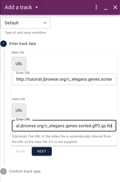

Using the admin-server to add a synteny track
http://tutorialpag31.jbrowse.org/c_elegans.c_brenneri.paf
