JBrowseR renders the JBrowse 2 linear genome view as an htmlwidget. JBrowse 2 is a fast, GPU-accelerated genome browser; JBrowseR lets you drive it entirely from R and embed it in R Markdown documents, Shiny apps, or the interactive console.
The API is declarative, and what you describe it with is
JBrowse’s own options: JBrowseR() takes
createLinearGenomeView’s options as named arguments, and
assemblies, tracks and sessions are the same JSON objects a
config.json holds, written as R lists. The package names
none of them, so an option, track type or view type JBrowse gains needs
nothing added here.
The one-liner
The fastest way in is to name a genome hub hosted at jbrowse.org. This gives you the assembly, reference-name aliases, cytobands, and gene-name search with no further setup:
JBrowseR(assembly = "hg38", location = "BRCA1")location accepts a region string like
"chr1:1-10000" or, because the hub ships a search index, a
gene name like "BRCA1". Other hubs work the same way —
"hg19", "mm10", or a GenArk accession such as
"GCF_000001405.40".
Adding tracks
Add tracks by URL with list(uri = ). The track type and
its index files (.bai/.crai/.tbi)
are inferred from the file extension, so a data URL is usually all you
need. list() gathers several together.
JBrowseR(
  assembly = "hg38",
  tracks = list(
    list(
    uri =
      "https://jbrowse.org/genomes/GRCh38/alignments/NA12878/NA12878.alt_bwamem_GRCh38DH.20150826.CEU.exome.cram",
      name = "NA12878 Exome"
    )
  ),
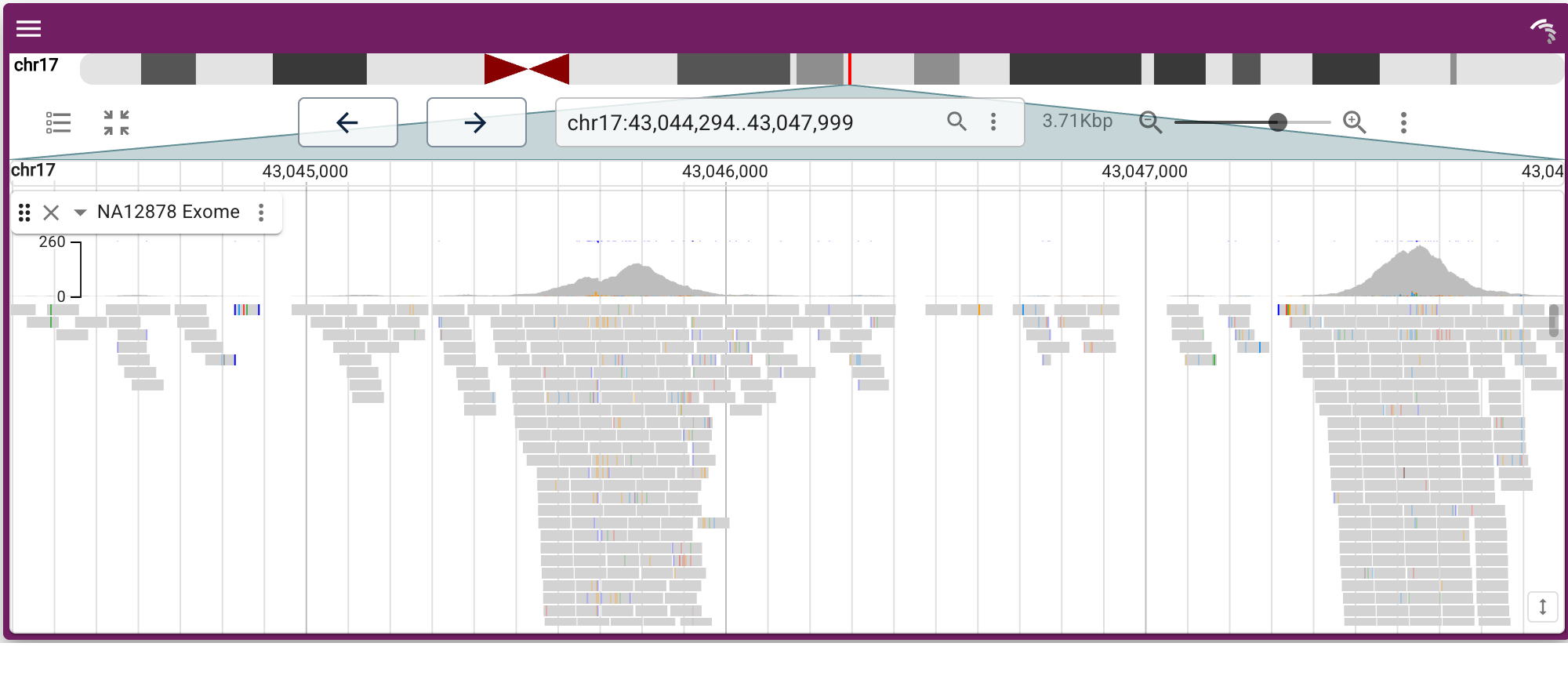
  location = "17:43,044,295..43,048,000"
)
Recognized extensions cover the common genomics types:
| Extension | Track | Adapter |
|---|---|---|
.bam, .cram
|
alignments |
BamAdapter, CramAdapter
|
.vcf.gz |
variants | VcfTabixAdapter |
.gff.gz, .gff3.gz, .gtf.gz,
.bed.gz
|
features |
Gff3TabixAdapter, GtfTabixAdapter,
BedTabixAdapter
|
.bb, .bigBed
|
features | BigBedAdapter |
.bw, .bigWig
|
quantitative | BigWigAdapter |
.hic |
Hi-C contact matrix | HicAdapter |
The list isn’t hard-coded in R — the view infers the adapter with
JBrowse’s own format plugins, so any format a bundled plugin recognizes
works. Anything the inference gets wrong, or a track needing a specific
adapter, is a plain config list (the full JBrowse track JSON); extra
arguments to list(uri = ) (e.g.
type = "AlignmentsTrack") ride onto the track and override
the inferred defaults.
When you only need the defaults, a bare URL string is a track —
list(uri = ) is just the same thing with room for
name= and extra config. So a whole browser can be a list of
URLs:
JBrowseR(
  assembly = "hg38",
  tracks = list(
    "https://hgdownload.soe.ucsc.edu/goldenPath/hg38/phyloP100way/hg38.phyloP100way.bw",
    "https://jbrowse.org/genomes/GRCh38/ncbi_refseq/GCA_000001405.15_GRCh38_full_analysis_set.refseq_annotation.sorted.gff.gz"
  ),
  location = "BRCA1"
)
Index files (.bai/.crai/.tbi)
default to the conventional sibling of the data URL. When yours lives
elsewhere — or is a .csi index — name it with
index=:
list(uri = "https://example.com/reads.bam", index = "https://example.com/reads.bai")A gallery
The figures below are screenshots, so this vignette stays small. Every one of them is also on the website as a live, interactive browser.
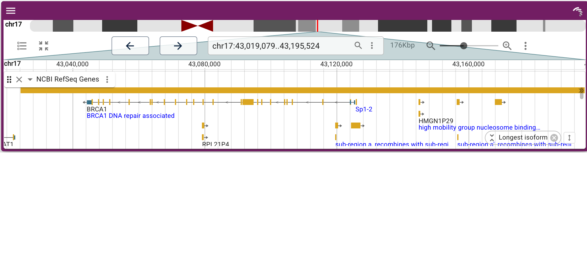
Genes. A gene annotation track over the hub assembly, navigated by name.
JBrowseR(
  assembly = "hg38",
  tracks = list(list(
    uri =
    "https://jbrowse.org/genomes/GRCh38/ncbi_refseq/GCA_000001405.15_GRCh38_full_analysis_set.refseq_annotation.sorted.gff.gz",
    name = "NCBI RefSeq Genes"
  )),
  location = "BRCA1"
)
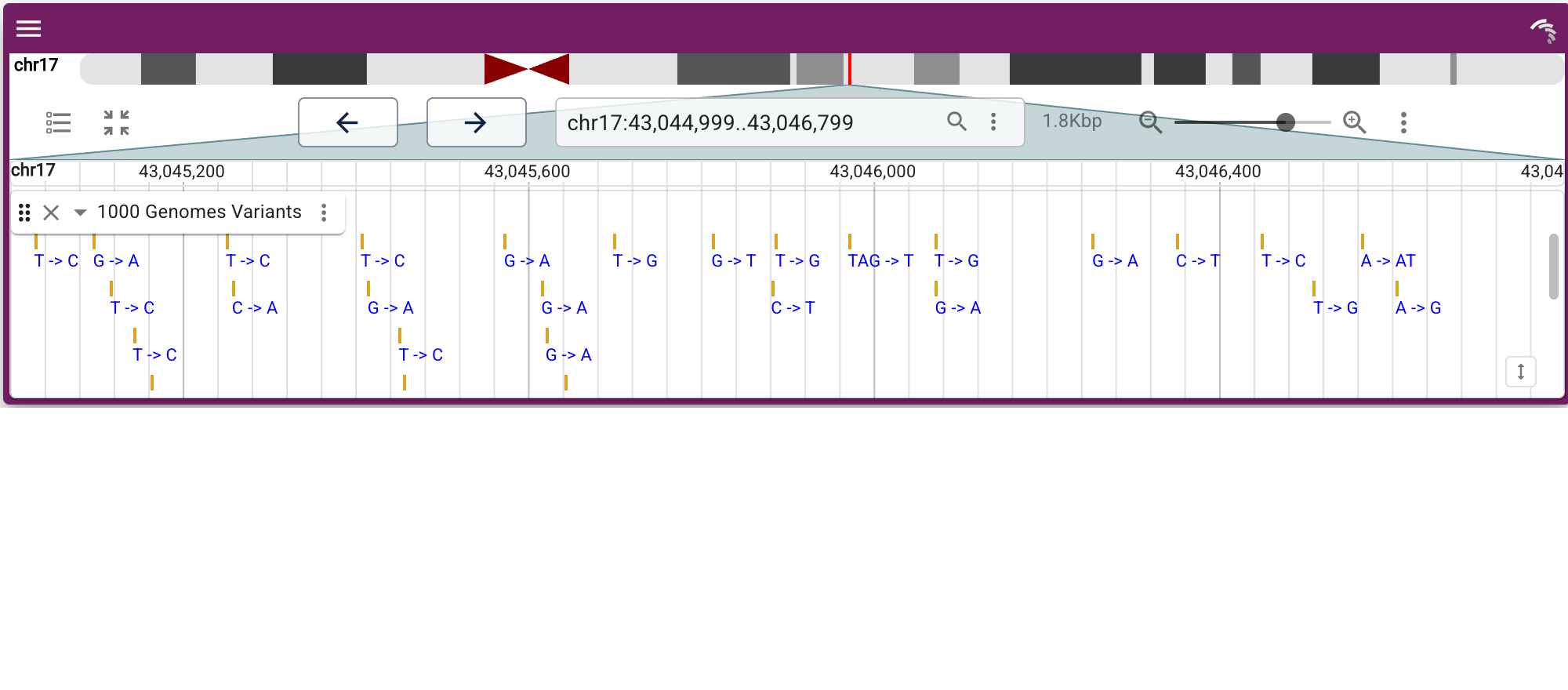
Variants. A 1000 Genomes VCF.
JBrowseR(
  assembly = "hg38",
  tracks = list(list(
    uri =
    "https://jbrowse.org/genomes/GRCh38/variants/ALL.wgs.shapeit2_integrated_snvindels_v2a.GRCh38.27022019.sites.vcf.gz",
    name = "1000 Genomes Variants"
  )),
  location = "17:43,045,000..43,046,800"
)
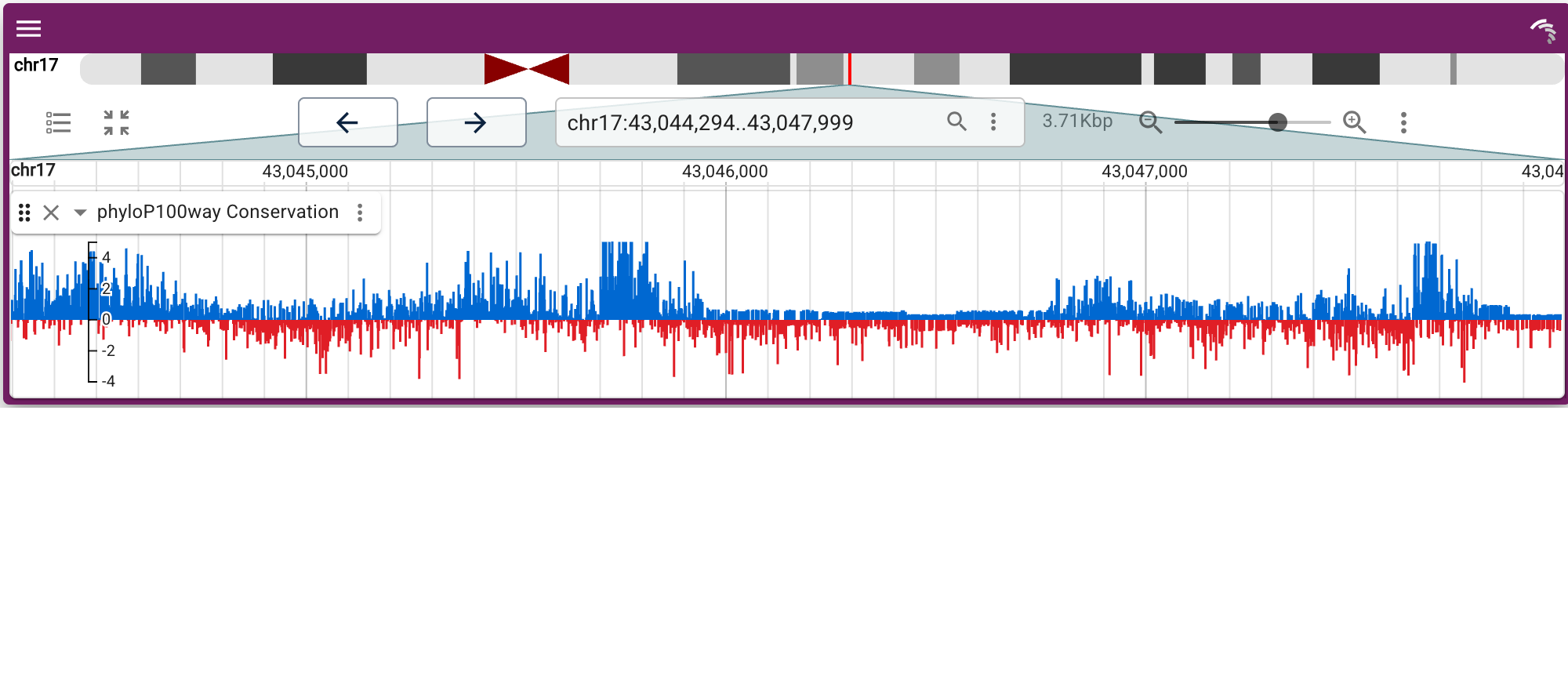
Quantitative. A phyloP conservation bigWig.
JBrowseR(
  assembly = "hg38",
  tracks = list(list(
    uri =
    "https://hgdownload.soe.ucsc.edu/goldenPath/hg38/phyloP100way/hg38.phyloP100way.bw",
    name = "phyloP100way Conservation"
  )),
  location = "17:43,044,295..43,048,000"
)
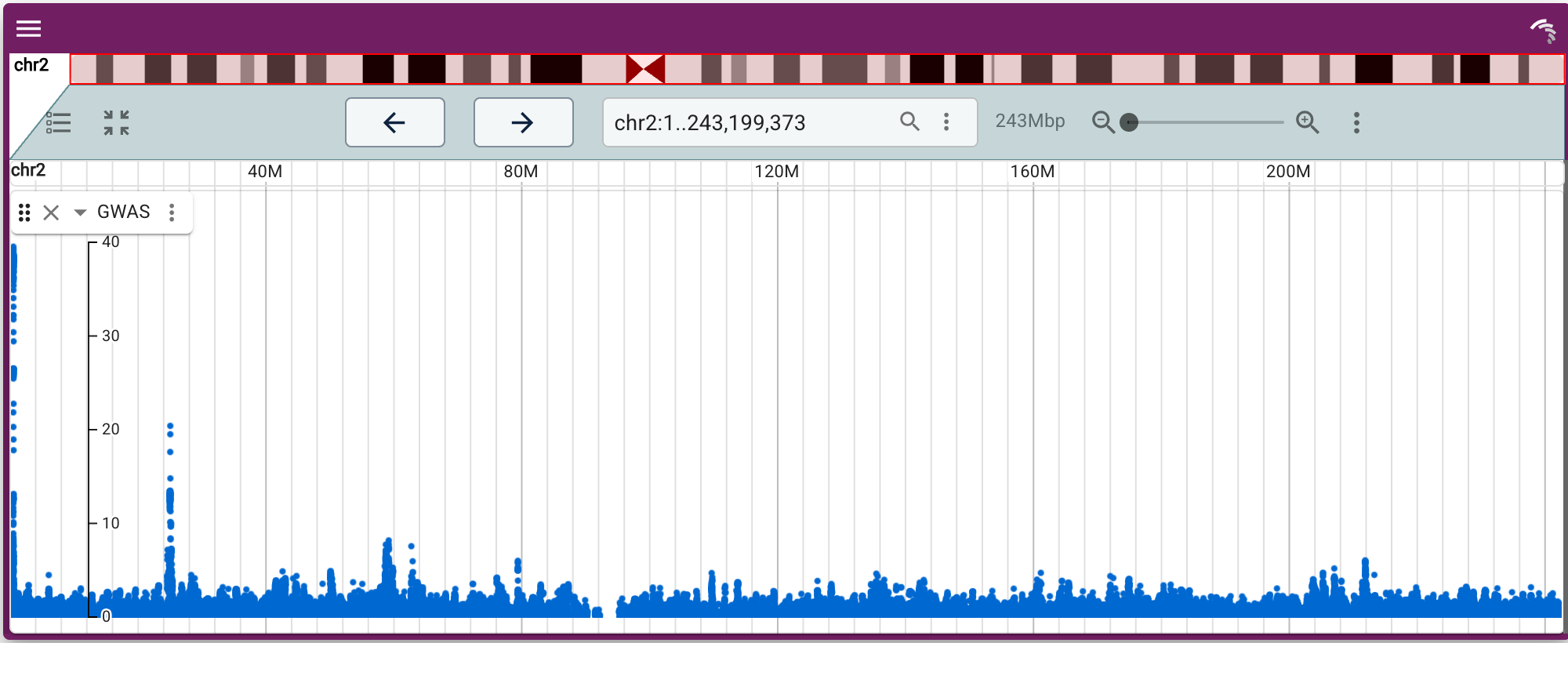
Plots from a display. A track’s display can
plot its data: a GWASTrack with a
LinearManhattanDisplay draws genome-wide summary statistics
as a Manhattan plot right in the linear view, so no separate plotting
widget is needed. Write the track as a config list — the same JSON a
JBrowse config file holds — and let the uri shorthand find
the .tbi index.
JBrowseR(
  assembly = "hg19",
  tracks = list(list(
    type = "GWASTrack",
    trackId = "gwas_track",
    name = "GWAS",
    adapter = list(
      type = "GWASAdapter",
      scoreColumn = "neg_log_pvalue",
      uri = "https://jbrowse.org/genomes/hg19/gwas/summary_stats.txt.gz"
    ),
    displays = list(list(type = "LinearManhattanDisplay", height = 250))
  )),
  location = "2"
)
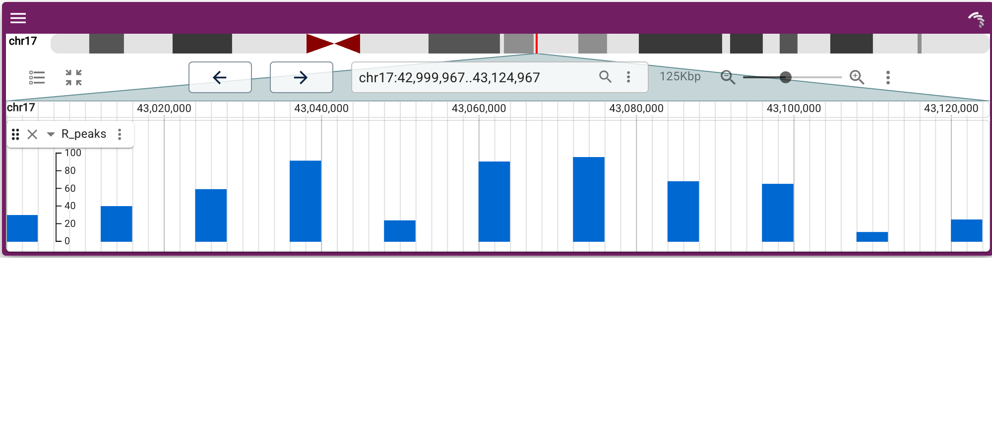
Your R results. Turn a data frame of features into a
track with track_data_frame() — no files and no web server.
Any score column makes it a quantitative track.
set.seed(1)
peaks <- data.frame(
  chrom = "17",
  start = seq(43000000, 43120000, by = 12000),
  end   = seq(43000000, 43120000, by = 12000) + 4000,
  name  = paste0("peak", 1:11),
  score = round(runif(11, 5, 100))
)

JBrowseR(
  assembly = "hg38",
  tracks = list(track_data_frame(peaks, "R_peaks")),
  location = "17:43,000,000..43,125,000"
)
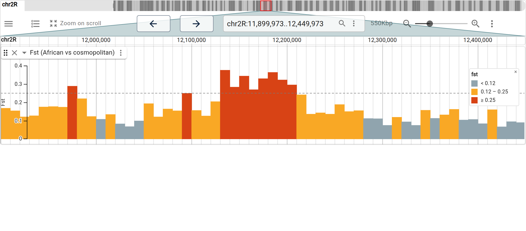
A plot from a data frame. A displays
entry says how to draw the rows, and LinearMarkDisplay is
JBrowse’s grammar of graphics: encoding maps columns to
channels the way aes() does, and the axis, legend and
reference lines come from the scales rather than from code. Here a
windowed Fst scan between two Drosophila populations, computed
in base R from hosted allele frequencies, is a bar per
window with fst on the value axis and a threshold colour
scale over the same column. The sweep at Cyp6g1 is the run of
bars past the 0.25 rule.
freqs <- read.csv("https://jbrowse.org/demos/popgen/dest_cyp6g1_freqs.csv")
p1 <- freqs$afr_freq
p2 <- freqs$cosmo_freq
window <- freqs$pos %/% 10000 * 10000
num <- tapply((p1 - p2)^2, window, sum)
den <- tapply(p1 * (1 - p2) + p2 * (1 - p1), window, sum)
fst <- data.frame(
  chrom = "chr2R",
  start = as.integer(names(num)),
  end = as.integer(names(num)) + 10000,
  fst = round(pmax(num / den, 0), 3),
  n_snps = as.vector(table(window))
)
fst <- fst[fst$n_snps >= 20, ]

JBrowseR(
  assembly = "dm6",
  tracks = list(track_data_frame(
    fst, "Fst (African vs cosmopolitan)",
    displays = list(list(
      type = "LinearMarkDisplay",
      scales = list(y = list(title = "Fst", rules = list(0.25))),
      marks = list(list(
        mark = "bar",
        encoding = list(
          y = "fst",
          color = list(
            field = "fst", scale = "threshold",
            domain = list(0.12, 0.25),
            range = list("#90a4ae", "#f9a825", "#d84315")
          )
        )
      ))
    ))
  )),
  location = "chr2R:11,900,000..12,450,000"
)
marks takes a bar, point or
span per entry, scale is
categorical, linear, log or
threshold, and a transform list can bin, count
or pack the rows first; the mark
display guide has the whole grammar. Every array in it is a
list(): rules = 0.25 would serialize as a
scalar.
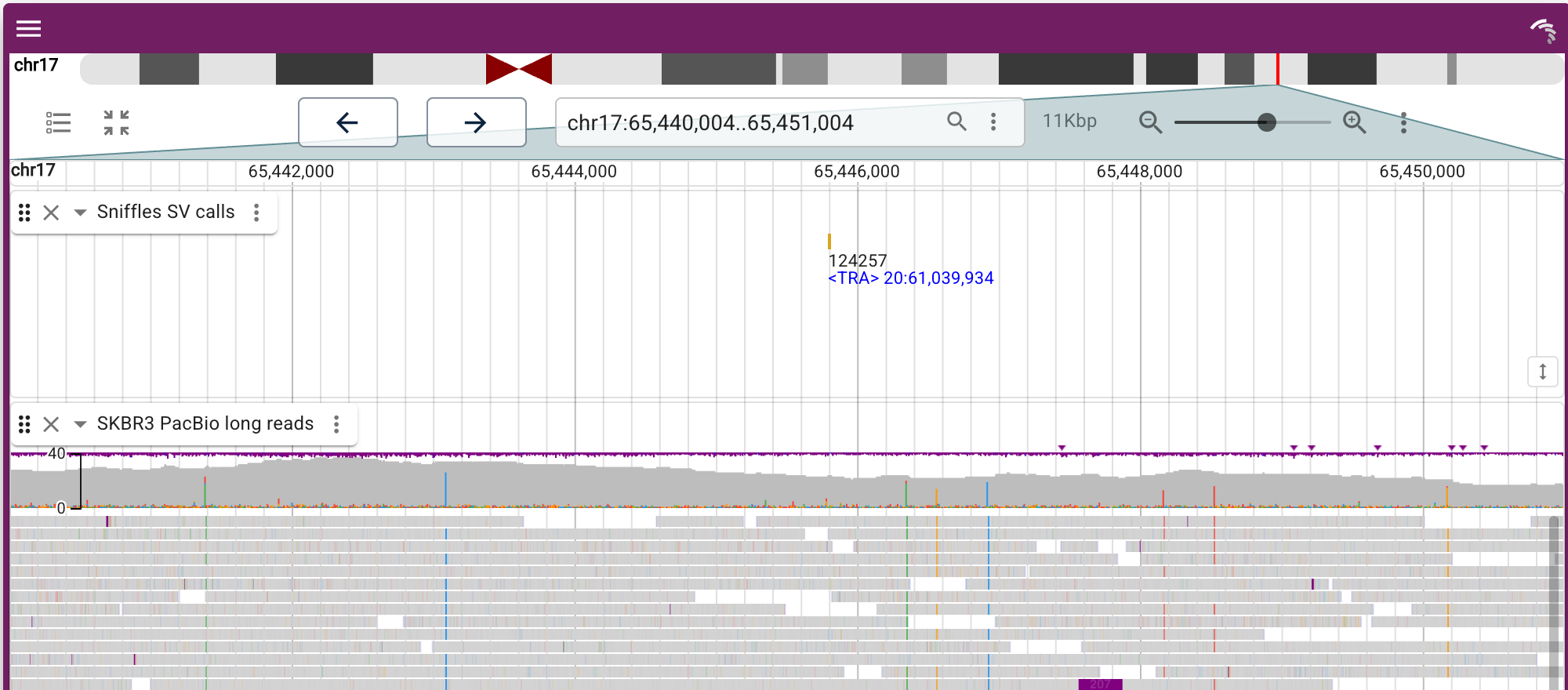
Cancer structural variants. The SKBR3 breast-cancer
cell line has a heavily rearranged genome. PacBio long reads span
breakpoints short reads cannot, and Sniffles calls the structural
variants from them. This view lands on a translocation from chr17 to
chr20 (<TRA> 20:61,039,934): the call sits in the
Sniffles track and the long reads carry it below.
JBrowseR(
  assembly = "hg19",
  tracks = list(
    list(
    uri =
      "https://jbrowse.org/genomes/hg19/SKBR3/reads_lr_skbr3.fa_ngmlr-0.2.3_mapped.bam.sniffles1kb_auto_l8_s5_noalt.filtered.vcf.gz",
      name = "Sniffles SV calls"
    ),
    list(
    uri =
      "https://jbrowse.org/genomes/hg19/skbr3/reads_lr_skbr3.fa_ngmlr-0.2.3_mapped.down.bam",
      name = "SKBR3 PacBio long reads"
    )
  ),
  location = "17:65,440,000..65,451,000"
)
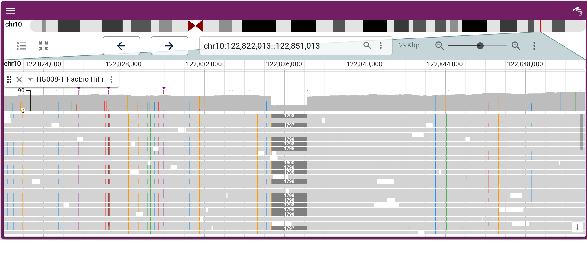
A somatic deletion. HG008-T is a tumor reference sample; its PacBio HiFi reads carry a ~1.8 kb somatic deletion in CUZD1, visible as a clean drop-out spanning many reads.
JBrowseR(
  assembly = "hg38",
  tracks = list(list(
    uri =
    "https://jbrowse.org/demos/cgiab/HG008-T_chr10_CUZD1_deletion.bam",
    name = "HG008-T PacBio HiFi"
  )),
  location = "10:122,822,000..122,851,000"
)
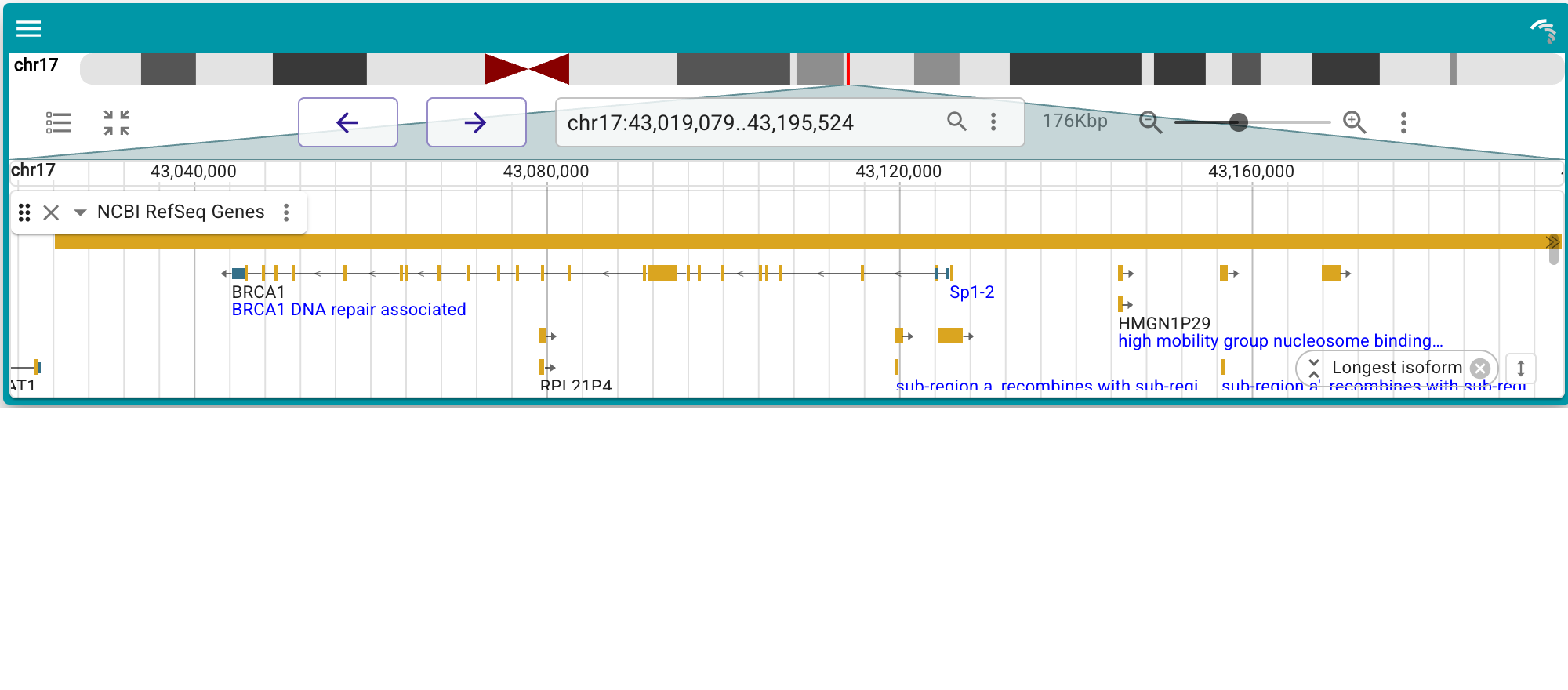
A custom theme. The theme slot of
JBrowse’s root configuration recolors the browser; it is
the MUI
palette JBrowse takes.
JBrowseR(
  assembly = "hg38",
  tracks = list(list(
    uri =
    "https://jbrowse.org/genomes/GRCh38/ncbi_refseq/GCA_000001405.15_GRCh38_full_analysis_set.refseq_annotation.sorted.gff.gz",
    name = "NCBI RefSeq Genes"
  )),
  configuration = list(theme = list(
    palette = list(
      primary = list(main = "#311b92"),
      secondary = list(main = "#0097a7")
    )
  )),
  location = "BRCA1"
)
Where to next
- A genome that isn’t on a hub? See the custom browser tutorial.
- Files on your own machine? See serving local data.
- Keeping a browser in a JSON file? See the JSON tutorial.
- Embedding in Shiny? Use
JBrowseROutput()andrenderJBrowseR(), read the selected feature back withinput$<outputId>_selected_feature, and navigate withupdate_jbrowse("<outputId>", location = loc).